Generate synthos data

The first version of synthos generates semi-realistic data of three benthic communities: hard coral, soft coral and macroalgae.

This vignette illustrates an example of how to use synthos by simulating observations of benthic communities using the following configuration:

Main configuration	Example settings
Observation data type	Point-based observations
Site allocation	Random locations
Number of sampling events	15 years
Sampling design	25 reefs, 3 sites per reef, 5 transects per site, 100 photo frames per transect, 50 points per frame, 2 depths
Relative disturbance weights	80% heat stress, 19% cyclone exposure, 1% other
Annual growth values	3% for hard coral and 3% for soft coral*

The configuration used in this example can be easily adjusted using the function generateSettings.

*Macroalgae responds differently: instead of growing independently, it occupies the remaining available space (i.e., macroalgae cover = total available space − (hard coral cover + soft coral cover) with total available space is fixed at 80% for each location).

Further explanations of each step can be found in the accompanying vignettes.

Setting up

# Load packages
library(sf)
library(stars)
library(gstat)
library(INLA)
library(ggplot2)
library(synthos)

1. Generate settings

surveys <-  "random" # or "fixed"
data_type <- "points" # or "cover"

synthos::generateSettings(nreefs = 25, nsites = 3, nyears = 15, dhw_eff = 0.5, cyc_eff = 0.3, other_eff = 0.2)

2. Generate the spatio-temporal domain, disturbance effects and baselines

spatial_domain <- st_geometry(
  st_multipoint(
    x = rbind(
      c(0, -11),
      c(3,-11),
      c(6,-14),
      c(1,-15),
      c(2,-12),
      c(0,-11)
    )
  )
) |>
  st_set_crs(config_sp$crs) |>
  st_cast("POLYGON")

## ---- SpatialPoints
set.seed(config_sp$seed)
spatial_grid <- spatial_domain |>
  st_set_crs(NA) |>
  st_sample(size = 10000, type = "regular") |>
  st_set_crs(config_sp$crs)
sf_use_s2(FALSE)

benthos_reefs_pts <- synthos::create_synthetic_reef_landscape(spatial_grid, config_sp)

3. Generate sampling design

if (surveys == "fixed") {
  locs_sf <- synthos::sampling_design_large_scale_fixed(
    benthos_reefs_pts, config_lrge
  )
  obs <- synthos::sampling_design_fine_scale_fixed(
    locs_sf, config_fine
  )
  
} else if (surveys == "random") {
  locs_sf <- synthos::sampling_design_large_scale_random(
    benthos_reefs_pts, config_lrge
  )
  obs <- synthos::sampling_design_fine_scale_random(
    locs_sf, config_fine
  )
} else {
  stop("surveys must be 'fixed' or 'random'.")
}

4. Generate export data table

if (data_type == "points") {
  pts <- synthos::sampling_design_fine_scale_points(obs, config_pt)
  synthos_data <- synthos::prepare_table(pts)  
  
} else if (data_type == "cover") {
  cov <- synthos::sampling_design_fine_scale_cover(obs, config_pt)
  synthos_data <- synthos::prepare_table(cov) 
  
} else {
  stop("data_type must be 'points' or 'cover'.")
}

5. Vizualisations

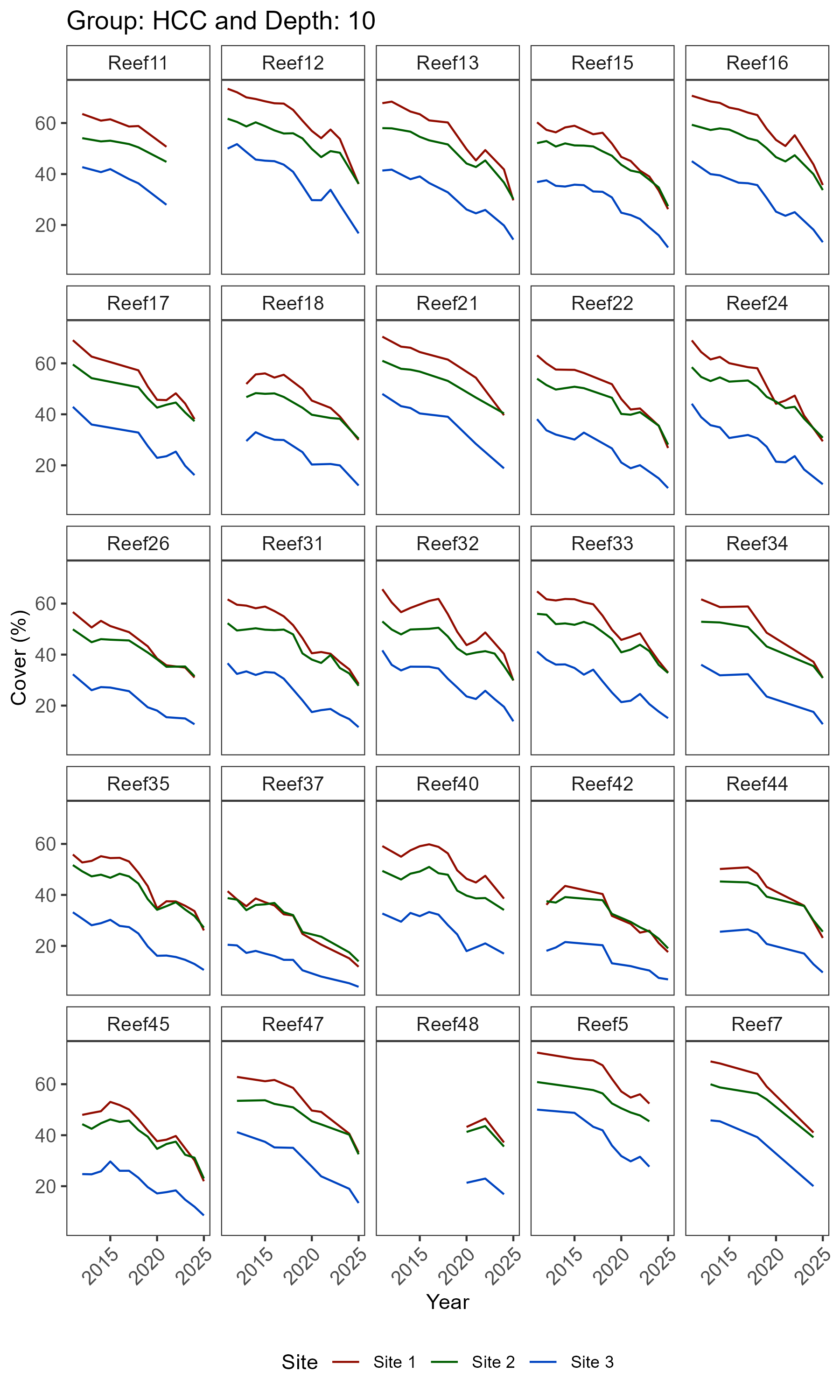
# 3.1 Long-term trajectories at site level

plots_1 <- synthos::plot_synthos(synthos_data, type = "trajectories")
purrr::walk(seq_along(plots), ~ ggsave(filename = paste0("figures/figure1.", .x, ".png"),
                                plot = plots[[.x]], width = 6, height = 10, dpi = 300))

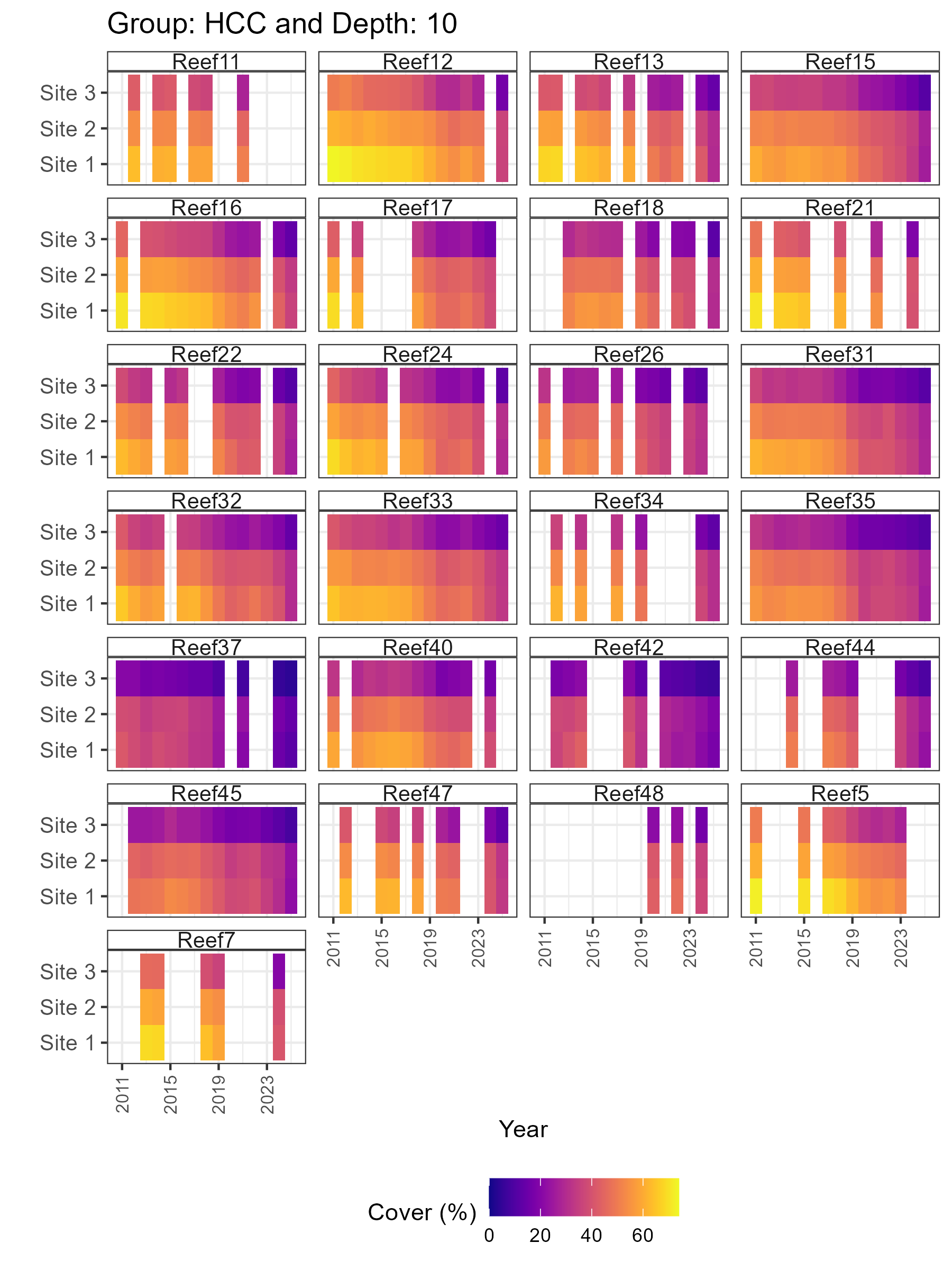
# 3.2 Heatmaps 
plots_2 <- synthos::plot_synthos(synthos_data, type = "heatmaps")
purrr::walk(seq_along(plots), ~ ggsave(filename = paste0("figures/figure2.", .x, ".png"),
                                plot = plots[[.x]], width = 6, height = 8, dpi = 300))

5.1 Trajectories

Figure 2: Trajectories of hard coral cover (HCC) at 10m depth.

5.2 Heatmaps

Figure 8: Temporal pattern of mean hard coral cover (HCC) by site at 10m depth.