Generate disturbances

Details on disturbances

synthos generates three types of disturbances known to reduce hard and soft coral cover. Each disturbance has its own spatial and temporal patterns, reflecting how these processes occur in reality.

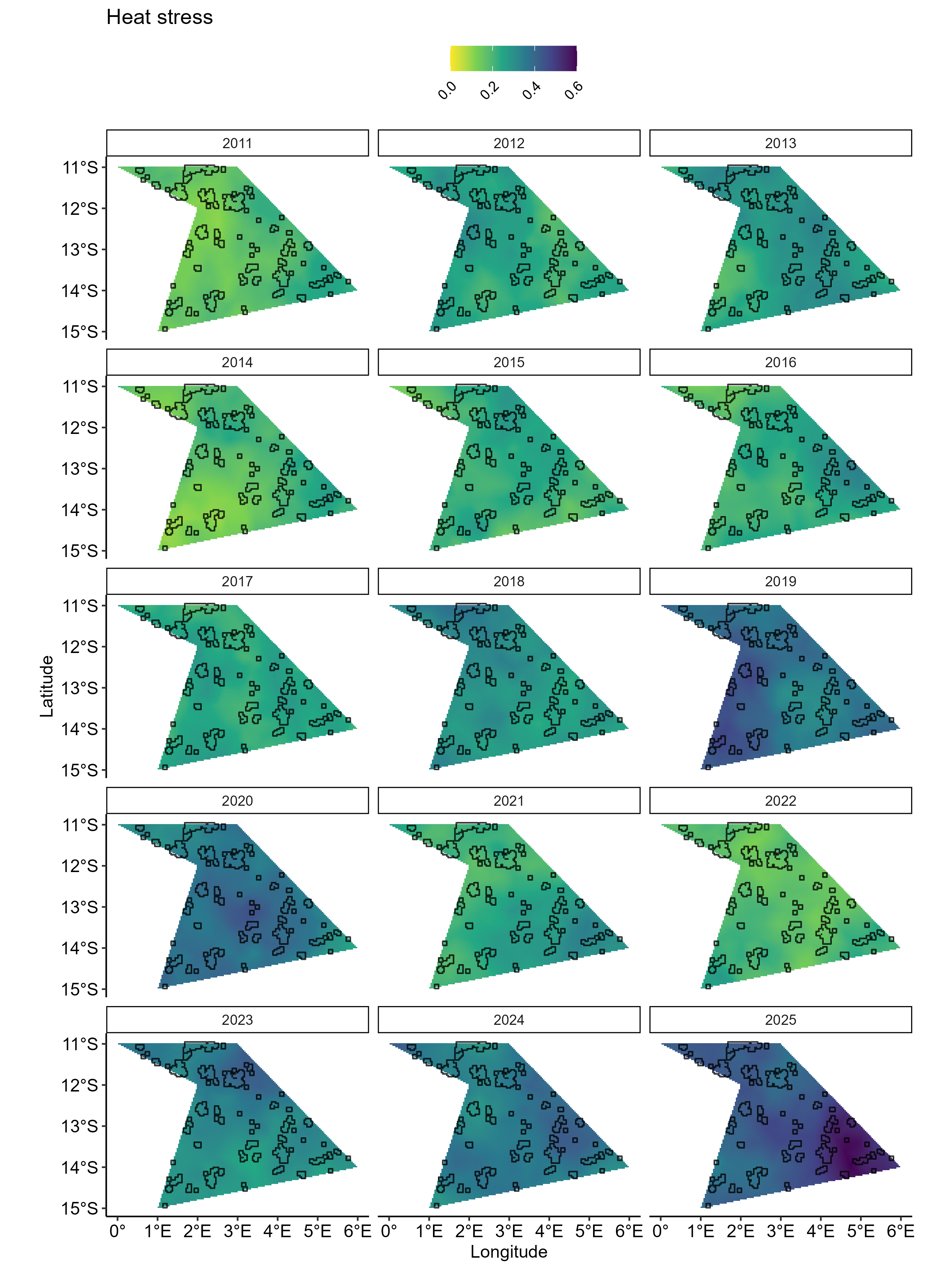
The intensity of a Heat stress event is approximated by the distribution of Degree Heating Weeks (DHWs) with maximum annual values correlated with mass coral bleaching and mortality. synthos modelled heat stress by first generating a temporal DHW signal that varies form year to year. Random values are then added to the trend to mimic the yearly variation of heat-stress events under long-term warming. The resulting temporal signal is then propagated across the spatial field using a time-varying AR(1)-like process and rescaled between [0-1] to support comparisons with other disturbances.

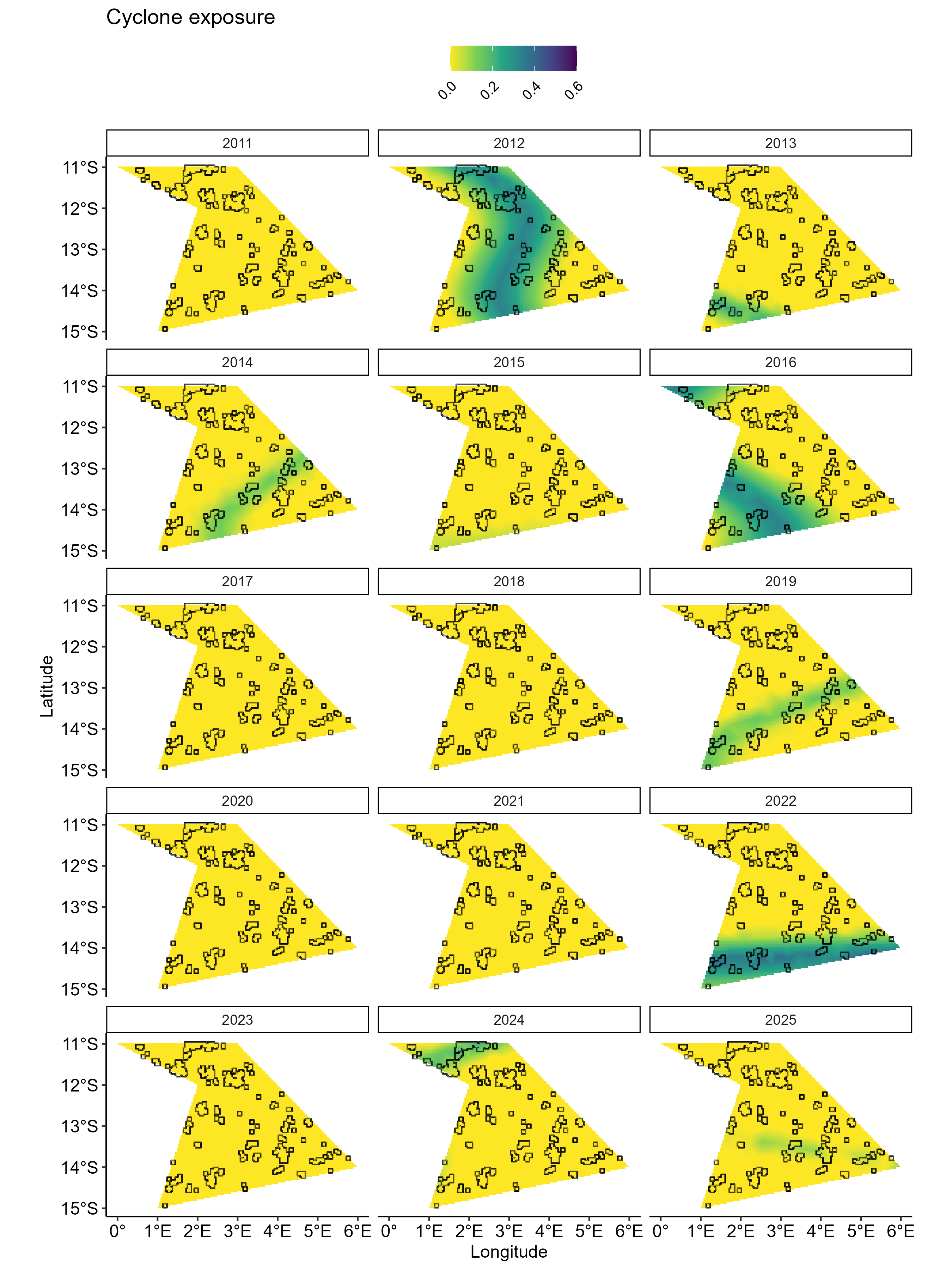
Exposure to Cyclones is modelled through three components:

• their occurrence
• their intensity
• the geographical effect: reflecting the fact that some locations are more susceptible to cyclone exposure than others

Cyclone occurrence in a given year is simulated as a binary event (yes/no) whose probability of happening increases through time. When a cyclone occurs, its intensity is also randomly generated from a probability distribution biased to produce stronger cyclone events on average. Values of cyclone intensity is then used to adjust the geographical effect to produce the fine spatial pattern of cyclone impact and rescaled between [0-1].

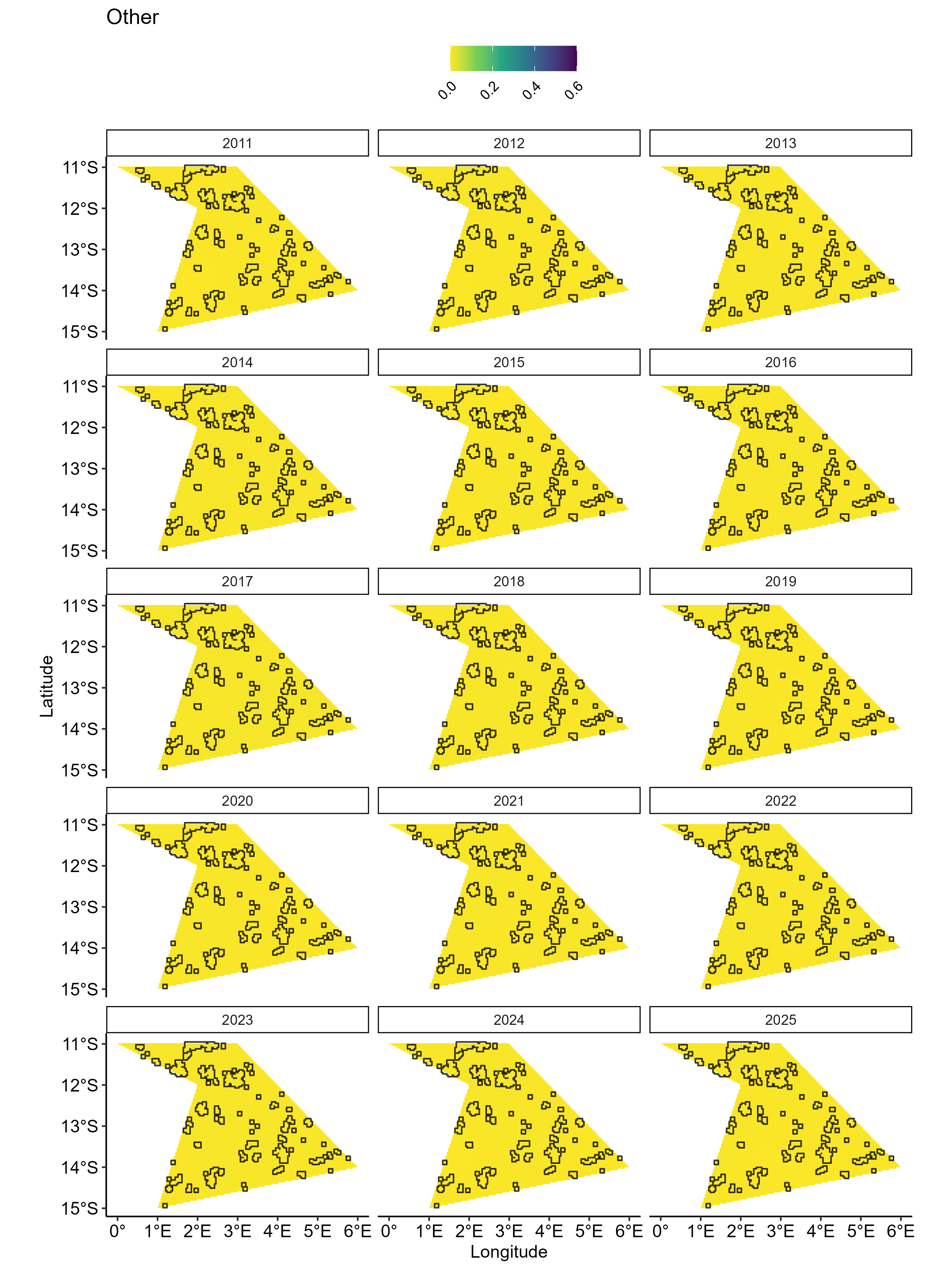
A third disturbance, Other, is generated using the same approach as heat stress disturbance but without the underlying temporal trend. Each year, spatial effects are drawn from a probability distribution parameterized to introduce low temporal autocorrelation values between consecutive years and rescaled between [0-1].

Details on the weighting system

Working with synthetic data requires the ability to recover the input values, including the effects of disturbances. Although disturbances are generated using both deterministic and stochastic processes, their influence can be controlled by applying weights. In synthos, disturbance values are scaled by user-defined deterministic weights, providing a simple and transparent way to modulate their impact. The configuration of the weights can be adjusted within the function generateSettings.

Setting up

# Load packages
library(sf)
library(stars)
library(gstat)
library(INLA)
library(ggplot2)
library(synthos)
library(stringr)
library(ggpubr)
library(scico)

1. Generate settings

surveys <-  "random" # or  "fixed"
data_type <- "points" # or "cover"

synthos::generateSettings(nreefs = 25, nsites = 3, nyears = 15, dhw_eff = 0.5, cyc_eff = 0.3, other_eff = 0.2)

1. Generate disturbances

spde <- synthos:::create_spde(spatial_grid, config_sp)

######### DHW 
dhw.pts.effects.df <- synthos:::disturbance_dhw(spatial_grid, spde, config_sp)$dhw_pts_effects_df %>%
                      mutate(Dist = "DHW") %>%
                      mutate(weight = config_sp$dhw_weight)
######### CYC
cyc.pts.effects <- synthos:::disturbance_cyc(spatial_grid, spde, config_sp)$cyc_pts_effects%>%
                      mutate(Dist = "CYC") %>%
                      mutate(weight = config_sp$cyc_weight)
########## OT
other.pts.effects <- synthos:::disturbance_other(spatial_grid, spde, config_sp)$other_pts_effects%>%
                      mutate(Dist = "OT")  %>%
                      mutate(weight = config_sp$other_weight)

########## All
all.pts.effects <- bind_rows(dhw.pts.effects.df, cyc.pts.effects, other.pts.effects) %>%
                      mutate(Value_weighted = Value * weight) %>%
                      arrange(Dist) %>%
                      mutate(Dist_plot = case_when(Dist == "DHW" ~ "Heat stress",
                                                   Dist == "CYC" ~ "Cyclone exposure",
                                                   Dist == "OT" ~ "Other")) %>%
                       dplyr::mutate(Year = as.numeric(format(Sys.Date(), "%Y")) - max(config_fine$years) + Year)

2. Vizualisation

effects_by_dist <- all.pts.effects %>%
  group_split(Dist)  

dist_levels <- all.pts.effects %>% distinct(Dist_plot) %>% pull(Dist_plot)

plots_by_dist <- map2(
  effects_by_dist,
  dist_levels,
  ~ ggplot() +  
      geom_tile(data = .x, aes(x = Longitude, y = Latitude, fill = Value_weighted)) +
      geom_sf(data = reefs.sf$simulated_reefs_sf, fill = NA, color = "black") +
      facet_wrap(~Year, ncol = 3)  +
      scale_fill_viridis_c(
        name = "",
        option = "viridis",
        direction = -1,
        na.value = "grey90",
        limits = c(0, 0.6),
        breaks = seq(0, 0.6, by = 0.2),
        labels = scales::number_format(accuracy = 0.1)
      ) +
      coord_sf(crs = 4326) +
      ggtitle(.y) +
      xlab("Longitude") +
      ylab("Latitude") +
      theme_pubr() +
      theme(
        legend.position = "top",
        legend.justification = c(0.5, 1),
        legend.direction = "horizontal",
        legend.text = element_text(angle = 45, hjust = 1),
        strip.background = element_rect(fill = 'white')
      )
)

Figure 1: Modelled relative and weighted exposure to cyclone across surveyed years.

Figure 2: Modelled relative and weighted heat stress across surveyed years.

Figure 3: Modelled relative and weighted other disturbances across surveyed years.