Generate baselines • synthos

In synthos, baselines represent the ecological community states in the year prior to sampling. In the current implementation, separate deterministic baseline surfaces are generated for hard coral (HCC) and soft coral (SC). Both baselines impose a west–east spatial gradient, with higher hard and soft coral cover in eastern locations, reflecting broad ecological patterns encoded through simple deterministic functions. The HCC and SC baselines differ primarily in how latitude influences cover. For hard corals (HCC), baseline values increase with latitude, whereas for soft corals (SC), a decreasing latitudinal effect is imposed. In addition, the rescaled baseline ranges are set higher for HCC than for SC, reflecting their comparatively greater expected cover in the initial state.

Setting up

# Load packages
library(sf)
library(stars)
library(gstat)
library(INLA)
library(ggplot2)
library(synthos)
library(stringr)
library(ggpubr)
library(scico)

1. Generate settings

surveys <-  "random" # or  "fixed"
data_type <- "points" # or "cover"

synthos::generateSettings(nreefs = 25, nsites = 3, nyears = 15, dhw_eff = 0.5, cyc_eff = 0.3, other_eff = 0.2)

2. Generate the baseline for hard corals


## ---- SyntheticData_Spatial.mesh
mesh <- synthos::create_spde_mesh(spatial_grid,config_sp)

## Synthetic Baselines ----------------------------------------------------
spatial.grid.pts.df <- spatial_grid %>%
  st_coordinates() %>%
  as.data.frame() %>%
  dplyr::rename(Longitude = X, Latitude = Y) %>%
  arrange(Longitude, Latitude)

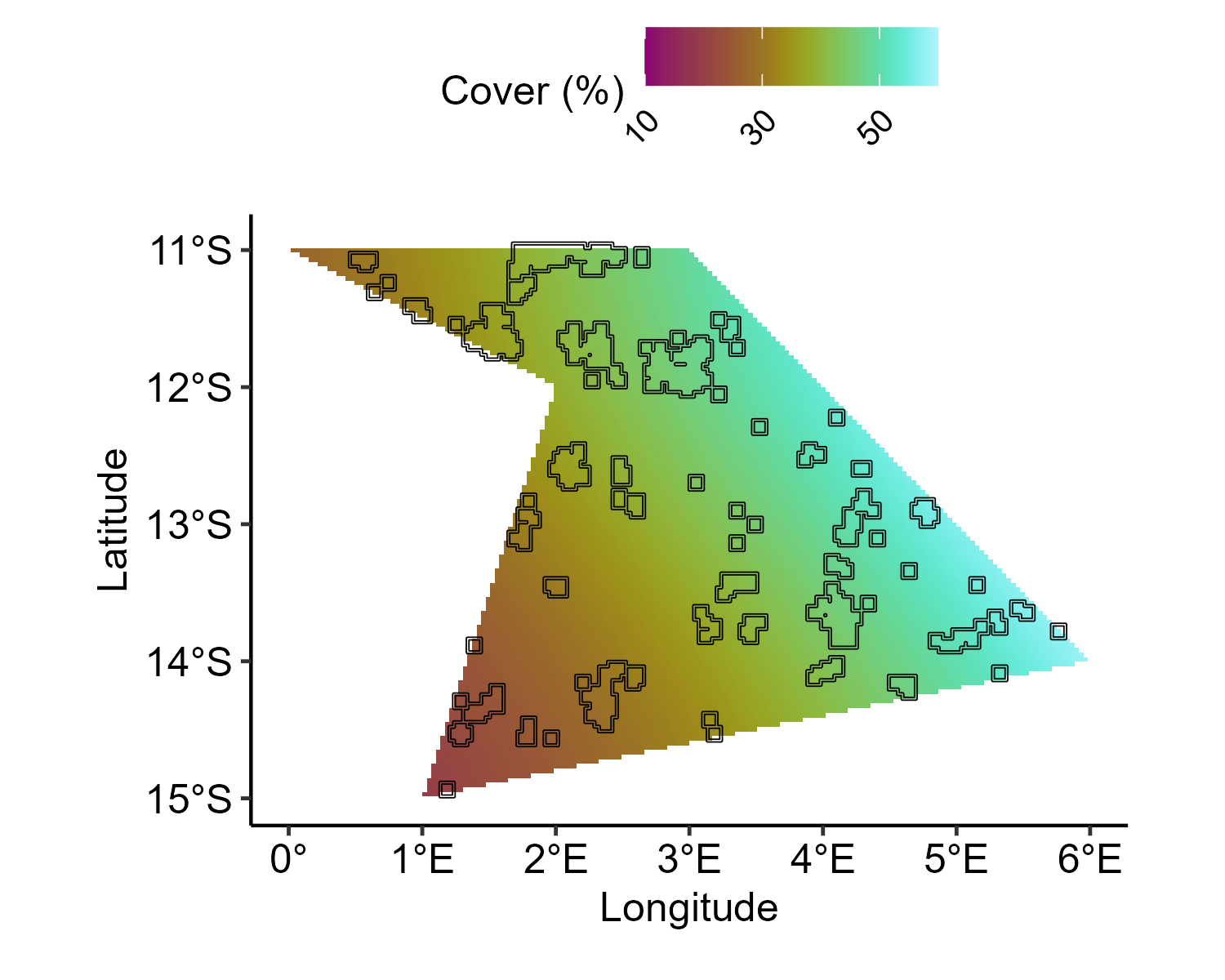
## ---- SyntheticData_BaselineSpatial.HCC

cover_range <- config_sp$hcc_cover_range
cover_range <- qlogis(cover_range)

baseline.sample.hcc <- mesh$loc[,1:2] %>%
  as.data.frame() %>%
  dplyr::select(Longitude = V1, Latitude = V2) %>%
  mutate(clong = as.vector(scale(Longitude, scale = FALSE)),
         clat = as.vector(scale(Latitude, scale = FALSE)),
         Y = clong + sin(clat) + 
           1.5*clong + clat) %>%
  mutate(Y = scales::rescale(Y, to = cover_range))

baseline.effects.hcc <- baseline.sample.hcc %>%
  dplyr::select(Y) %>%
  as.matrix
baseline.pts.sample.hcc <- inla.mesh.project(mesh,
                                             loc=as.matrix(spatial.grid.pts.df [,1:2]),
                                             baseline.effects.hcc)
baseline.pts.effects.hcc = baseline.pts.sample.hcc %>% 
  cbind() %>% 
  as.matrix() %>% 
  as.data.frame() %>%
  cbind(spatial.grid.pts.df ) %>% 
  pivot_longer(cols = c(-Longitude,-Latitude),
               names_to = c('Year'),
               names_pattern = 'sample:(.*)',
               values_to = 'Value') %>%
  mutate(Year = as.numeric(Year))

ggplot() +
  geom_tile(
    data = baseline.pts.effects.hcc, 
    aes(y = Latitude, x = Longitude, fill = 100 * plogis(Value))
  ) +
  geom_sf(
    data = reefs.sf$simulated_reefs_sf, 
    fill = NA, 
    color = "black"
  ) +
  scico::scale_fill_scico(
    "Coral cover (%)",
    palette = "hawaii",      
    direction = 1,
    limits = c(10, 60),        
    breaks = seq(10, 60, by = 20),
    labels = scales::number_format(accuracy = 1)
  ) +
  coord_sf(crs = 4326) +
  xlab("Longitude") + 
  ylab("Latitude") +
  theme_pubr() +
  theme(
    legend.position = "top",
    legend.justification = c(0.5, 1),
    legend.direction = "horizontal",
    legend.text = element_text(angle = 45, hjust = 1)
  )

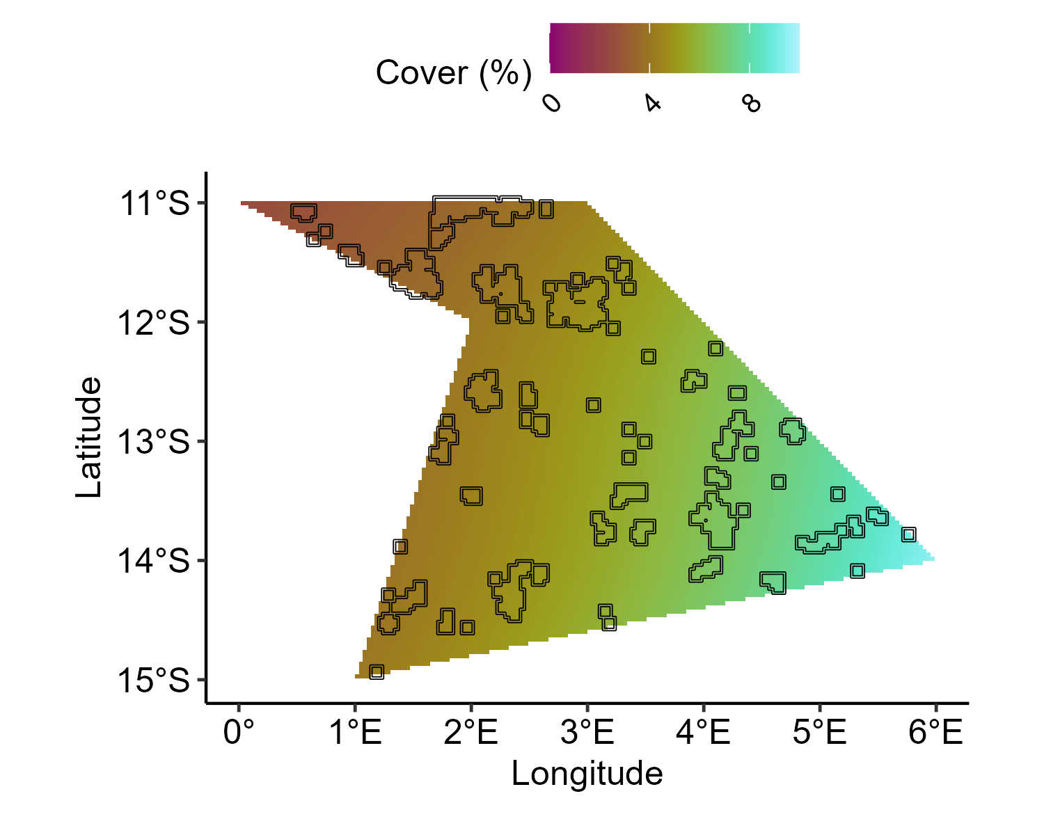
Coral reef — Figure 1: Baseline values for hard corals.

3. Generate the baseline for soft corals


cover_range <- config_sp$sc_cover_range
cover_range <- qlogis(cover_range)

baseline.sample.sc <- mesh$loc[, 1:2] %>%
  as.data.frame() %>%
  dplyr::select(Longitude = V1, Latitude = V2) %>%
  mutate(
    clong = as.vector(scale(Longitude, scale = FALSE)),
    clat = as.vector(scale(Latitude, scale = FALSE)),
    Y = clong + sin(clat) +
      1.5 * clong + -1.5 * clat
  ) %>%
  mutate(Y = scales::rescale(Y, to = cover_range))

baseline.effects.sc <- baseline.sample.sc %>%
  dplyr::select(Y) %>%
  as.matrix()
baseline.pts.sample.sc <- inla.mesh.project(mesh,
  loc = as.matrix(spatial.grid.pts.df [, 1:2]),
  baseline.effects.sc
)
baseline.pts.effects.sc <- baseline.pts.sample.sc %>%
  cbind() %>%
  as.matrix() %>%
  as.data.frame() %>%
  cbind(spatial.grid.pts.df) %>%
  pivot_longer(
    cols = c(-Longitude, -Latitude),
    names_to = c("Year"),
    names_pattern = "sample:(.*)",
    values_to = "Value"
  ) %>%
  mutate(Year = as.numeric(Year))

ggplot() +
  geom_tile(
    data = baseline.pts.effects.sc, 
    aes(y = Latitude, x = Longitude, fill = 100 * plogis(Value))
  ) +
  geom_sf(
    data = reefs.sf$simulated_reefs_sf, 
    fill = NA, 
    color = "black"
  ) +
  scico::scale_fill_scico(
    "Cover (%)",
    palette = "hawaii",      
    direction = 1,
    limits = c(0, 10),        
    breaks = seq(0, 10, by = 4),
    labels = scales::number_format(accuracy = 1)
  ) +
  coord_sf(crs = 4326) +
  xlab("Longitude") + 
  ylab("Latitude") +
  theme_pubr() +
  theme(
    legend.position = "top",
    legend.justification = c(0.5, 1),
    legend.direction = "horizontal",
    legend.text = element_text(angle = 45, hjust = 1)
  )