Example workflow¶

import cost_eco_model_linker as ceml

# Filepath to RME runs to process
rme_files_path = "./data/eco_linker_example"
deployment_model = "./3.5.5 CA Deployment Model"
production_model = "./3.7.0 CA Production Model"
output_path = "./results"
unc_config = ceml.default_uncertainty_dict()

# Change the entries in `unc_config` if needed
# unc_config["rti_uncert"] = 0

# Number of sims for metrics sampling (default includes ecological and expert uncertainty in RCI calcs)
nsims = 10

ceml.evaluate(
    rme_files_path,
    nsims,
    deployment_model,
    production_model,
    output_path,
    uncertainty_dict=unc_config,
)

For parallel runs:

nsims = 10
ncores = 4

if __name__ == "__main__":
    ceml.parallel_evaluate(
        rme_files_path,
        nsims,
        ncores,
        deployment_model,
        production_model,
        output_path,
        uncertainty_dict=unc_config,
    )

Sensitivity analysis¶

import cost_eco_model_linker as ceml

prod_cost_model = "./models/3.9.1 CA Production Model.xlsx"
deploy_cost_model = "./models/3.9.0 CA Deployment Model.xlsx"

# Number of samples to take (must be power of 2)
N = 2**7

# Samples model and returns an SALib problem specification with results under the
# `cost_model_results` key.
prod_sp = ceml.run_production_model(prod_cost_model, N)
deploy_sp = ceml.run_deployment_model(deploy_cost_model, N)

# Conduct and save sensitivity analysis results
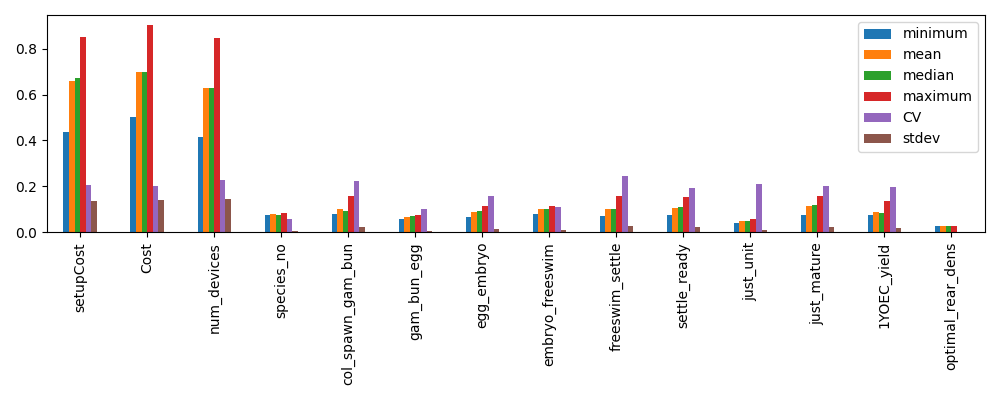
ceml.extract_sa_results(prod_sp, "./figs/prod/")
ceml.extract_sa_results(deploy_sp, "./figs/deploy/")

The above will generate a set of figures (for production or deployment costs).

Example PAWN analysis results:

PAWN SA barplot

Running models directly¶

The model type (production or deployment) and config version are inferred automatically from the workbook filename, so you only need to supply the path.

Single evaluation¶

evaluate_production_cost and evaluate_deployment_cost accept keyword arguments for any factor you want to override; all other factors default to the values currently in the spreadsheet. Both return (capex, opex).

import cost_eco_model_linker as ceml

production_model = "./models/3.9.1 CA Production Model.xlsx"
deployment_model = "./models/3.9.0 CA Deployment Model.xlsx"

capex, opex = ceml.evaluate_production_cost(production_model, num_1yoec=1_000_000)
print(capex + opex)

capex, opex = ceml.evaluate_deployment_cost(deployment_model, reef=2, distance_from_port=40)
print(capex + opex)

Batch evaluation¶

run_cost_model accepts a DataFrame where each row is one model evaluation. Columns not present default to the values in the spreadsheet.

import pandas as pd
import cost_eco_model_linker as ceml

production_model = "./models/3.9.1 CA Production Model.xlsx"

samples = pd.DataFrame({
    "num_1yoec": [500_000, 1_000_000, 2_000_000],
    "coral_yield_1YOEC": [0.3, 0.4, 0.5],
    "species_no": 20,
})

# Serial
results = ceml.run_cost_model(production_model, samples)

# Parallel — each worker opens its own temporary copy of the workbook
if __name__ == "__main__":
    results = ceml.run_cost_model(production_model, samples, nprocs=4)

#    num_1yoec  coral_yield_1YOEC  species_no      capex       opex  total_cost
# 0     500000                0.3          20  2696740.0   910485.3   3607225.3
# 1    1000000                0.4          20  4411200.0  1473854.1   5885054.1
# 2    2000000                0.5          20  6788400.0  2530646.0   9319046.0

Parameter sweep¶

run_parameter_sweep evaluates both models over a range of values for a single parameter, keeping all other factors at their spreadsheet defaults.

import numpy as np
import cost_eco_model_linker as ceml

production_model = "./models/3.9.1 CA Production Model.xlsx"
deployment_model = "./models/3.9.0 CA Deployment Model.xlsx"

# Sweep num_1yoec, all other factors at spreadsheet defaults
df = ceml.run_parameter_sweep(
    production_model,
    deployment_model,
    sweep_param="num_1yoec",
    search_range=range(100_000, 500_000, 100_000),
)

# Fix additional production factors while sweeping coral_yield_1YOEC
df = ceml.run_parameter_sweep(
    production_model,
    deployment_model,
    sweep_param="coral_yield_1YOEC",
    search_range=np.arange(0.3, 0.51, 0.1),
    prod_params={"num_1yoec": 1_000_000, "species_no": 20},
)
#    search_range  prod_capex    prod_opex  dep_capex      dep_opex        totals
# 0           0.3   5393480.0  1820970.500  1320560.0  7.870774e+06  1.640578e+07
# 1           0.4   4411200.0  1473854.125  1320560.0  7.870774e+06  1.507639e+07
# 2           0.5   3394200.0  1265323.000  1320560.0  7.870774e+06  1.385086e+07

Questions and Answers¶

How are deployment distances determined?¶

For a given simulation, a set of reefs where interventions occur are determined a priori, or as part of a simulated dynamic decision making process.

The mean longitude and latitude is determined for a defined set of intervention locations. From this, the distance to the closest port is determined.

While CEML does not currently support assessment of deployment scenarios that change deployment locations throughout a simulation, the determined costs should still be representative/indicative so long as the intervention reefs are confined within a given area.

What does `discrete_values` column in the configuration CSV do?¶

The flooring trick is used to map an input from its continuous sampled representation back to a discrete value. This naturally works when the inputs are intended to be between whole numbers (e.g., 1, 2, 3), but non-Real discrete values (e.g., 0.1, 0.2, 0.3) are trickier. To handle this, the discrete_values column samples between the number of available options and the sampled value then mapped back to the option value:

Parameter range: 0.1 to 0.5, incrementing by 0.1
Sampled range: 1 - 5

Sampled values are continuous:
[1.145, 2.11, 3.24, 4.34, 5.21]

Taking the floor of the sample resolves to:
[1.0, 2.0, 3.0, 4.0, 5.0]

Based on a mapping:
1 -> 0.1
2 -> 0.2
3 -> 0.3
4 -> 0.4
5 -> 0.5

So the realized sample is then:
[0.1, 0.2, 0.3, 0.4, 0.5]

How are distances between production facility and port handled?¶

The current implementation is to identify the center location of all intervention reefs, and then to identify the closest representative reef (as configured in the cost models). From there, the closest representatative port is identified. This port is what is used to indicate the facility-port distance.

An alternate conceptualization is that ports may be too busy, or operators unavailable. In such circumstances, it is plausible that an different port would be used. The line below could be added to the deployment configuration CSV to explore such scenarios.

deployment,Dashboard,D17,distance_from_facility,integer,50,350,50,50,350,“50,350”,discrete,TRUE,in kilometers