Introduction to MixMustR
Diego Barneche and Chris Fulton
2025-06-23
Source:vignettes/introduction.Rmd
introduction.RmdOverview
MixMustR is a flexible Bayesian mixture model package
written in the probabilistic programming language Stan for R. It estimates source mixing
proportions by incorporating simultaneous likelihood evaluation from two
independent data streams collected from the mixture of interest:
- Chemical tracers/biomarkers (e.g., stable isotopes, fatty acids).
- Source composition (e.g., based on eDNA or metabarcoding).
MixMustR also allows for the estimation of an
additional, unsampled source component to partially relax the assumption
that the mixing proportions from all sampled sources should sum to 1.
This makes it particularly useful in ecological studies, such as
understanding carbon source-sink dynamics or trophic interactions.
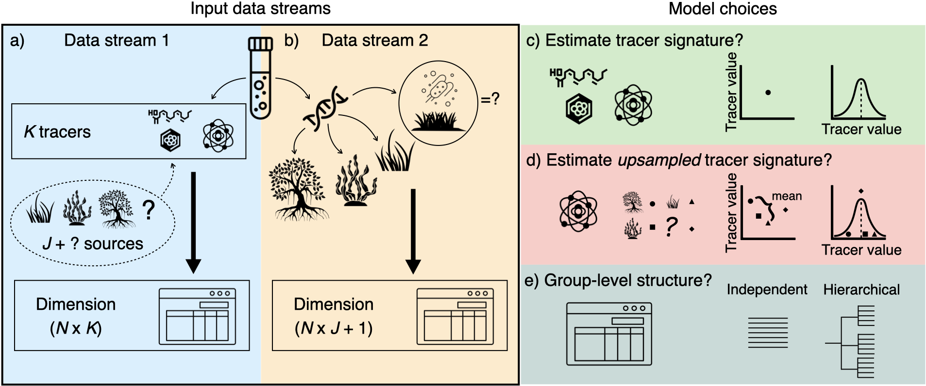
Figure 1: MixMustR input data and
framework.
This vignette will walk you through the basic usage of
MixMustR, covering:
- Preparing input data
- Running multiple model configurations
- Visualizing model fit
Model Variants
MixMustR provides eight model variants based on three
user-driven binary choices:
-
Tracer signature error structure:
- Residual-only error (similar to MixSIAR).
- Process error (incorporates uncertainty in tracer signatures).
-
Unsampled-source tracer signatures:
- Fixed at the mean across sampled sources.
- Estimated using a prior informed by sampled tracer signatures.
-
Observation independence:
- Independent observations.
- Hierarchical grouping structure.
The combination of these three choices is pre-packaged in
MixMustR via the data frame
mixmustr_models.
Synthetic Datasets in MixMustR
The MixMustR package includes two synthetic mixture
datasets, synthetic_df_convergent and
synthetic_df_divergent, designed for testing and validation
purposes. Both datasets are anchored to empirical values of stable
isotopes and fatty acids from plant carbon sources in marine soils and
simulate a hierarchical, unbalanced ecological field sampling
design.
-
synthetic_df_convergent: Exhibits minimal differences in the underlying mixing proportions between data streams 1 and 2. -
synthetic_df_divergent: Exhibits significant differences in the underlying mixing proportions between data streams 1 and 2.
Each dataset is a list containing three data frames:
df_stream_1: Simulated mixture data for the first stream, including tracer estimates. Its size is N observations by K tracers. It also contains an additional column namedgroup, which captures the grouping structure of this synthetic dataset. This group column is not mandatory, e.g., in case all observations are independent.df_stream_2: Synthetic proportions for the second stream, with a column for each source. Its size is N observations by J sources. At the observation/row level, the sum should be constrained between 0 and 1. Likedf_stream_1, it also contains an additional column namedgroup, which captures the grouping structure of this synthetic dataset.stream_1_props: Synthetic proportions for the first stream. This data frame is not a mandatory requirement to run models inMixMustR, it is only exported and used for testing purposes.
These datasets and their underlying simulated synthetic proportions
were generated using internal non-exported functions, combining data
from stable isotopes (bcs_si) and fatty acids
(bcs_fa). These synthetic datasets are valuable for
evaluating the ability of model variants to retrieve underlying mixture
proportions, and MixMustR offers diagnostic tools available
for summary and visualization.
Setup
We begin by loading the package and setting options for parallel computing and Stan:
library(MixMustR)
rstan::rstan_options(auto_write = TRUE)
options(mc.cores = parallel::detectCores())
Step 1: Prepare Tracer Parameters
We’ll assume you have access to source tracer summaries—mean
(mus), standard deviation (sigmas) and sample
size (ns) values for each source. These should be combined
into a named list, and MixMustR provides an example list
called tracer_parameters.
These are required to inform the model about each source’s chemical signatures and the variability around them.
Step 2: Run the Models
The core function to run models is
run_mixmustr_models(). This function allows you to run
multiple models defined in the built-in mixmustr_models
data frame. In addition to the model(s) of choice, the user also needs
the input data frame (here we use the synthetic dataset
synthetic_df_convergent), and declare their level of
confidence in the input mixing proportions of data stream 2 via the
parameter sigma_ln_rho. MixMustR transforms
the mixing proportions from data stream 2 before running a model, and
sigma_ln_rho captures the measurement error on the latent
log-transformed mixing proportion, and in practice can be interpreted as
the degree of confidence a user has in each element of log-transformed
mixing proportions from data stream 2.
model_fits <- run_mixmustr_models(
  mixmustr_models[6, ], synthetic_df_convergent, tracer_parameters,
  sigma_ln_rho = 1, iter = 1e4, warmup = 5e3, chains = 4, cores = 1
)
Importantly, MixMustR ingests that confidence at the observation
and source level. If the user inputs a single numeric value for
sigma_ln_rho as above, that will be applied across all
observations in data stream 2. Choosing the appropriate value for the
uncertainty around data stream 2 is not trivial. Therefore, the
MixMustR package offers a simple tool which plots the
expected variability in mixing proportion as a function of an input
vector of mixing proportions from data stream 2 (one from each source),
and their respective degrees of confidence or measurement error.
Although the function does not inform the user what the expected
uncertainty for each source and observation should be (what has to come
from expect knowledge), it does allow the user to fine tune
sigma_ln_rho until the appropriate variability in input
mixing proportions is achieved. As an example, we show the expected
variability in mixing proportions that would result from the value of 1
above:
# An observation from input mixing proportion in data stream 2, remove the group
#  column.
pis <- unlist(synthetic_df_convergent$df_stream_2[2, -1])
# Then for each create a value for their measurement error
sigma_ln_rho <- rep(1, length(pis))
# Visualize the potential parameter resulting from the chosen uncertainty
MixMustR::evaluate_uncertainty(pis, sigma_ln_rho)$plot
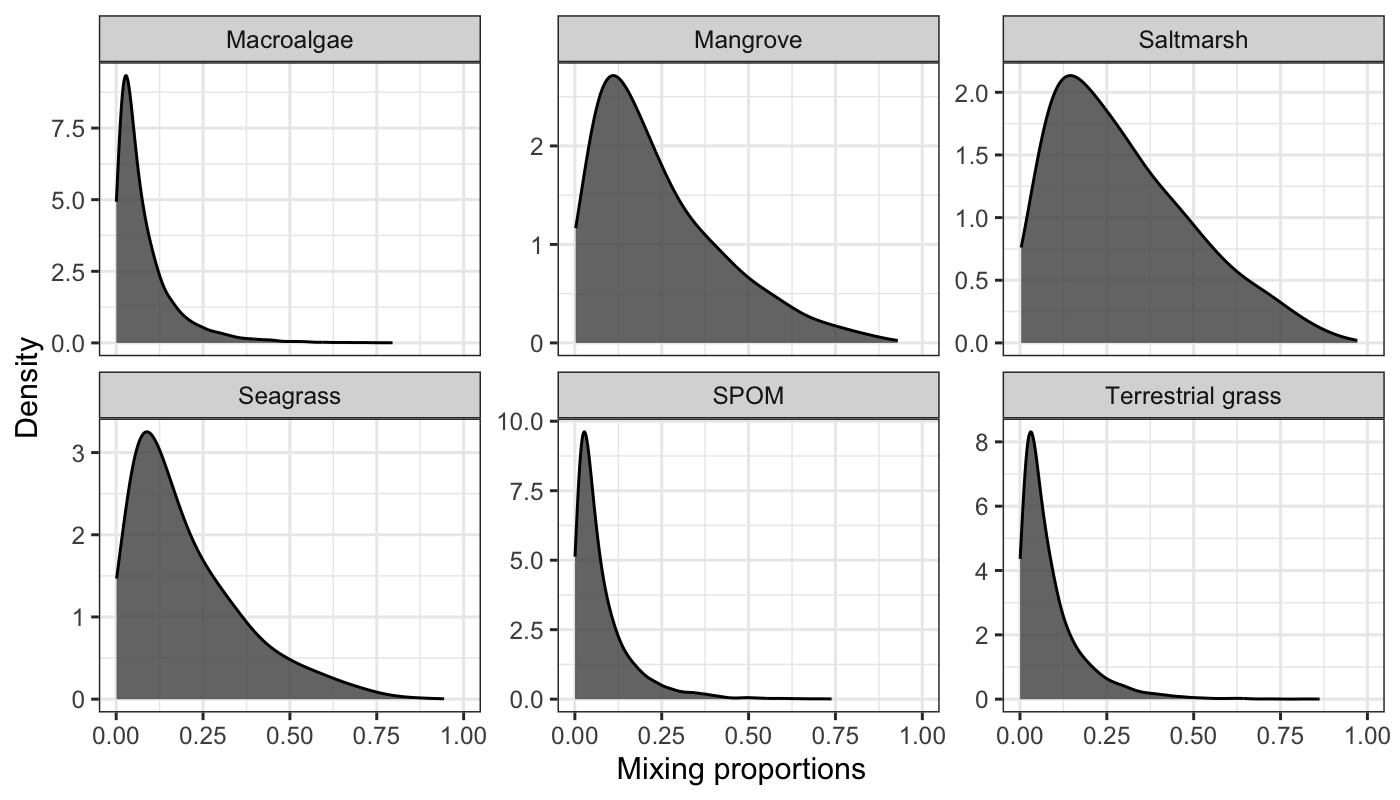
So a decent amount of variation is allowed with this value. This could reflect, for example, weak confidence in the mixing proportion observations in data stream 2.
Behind the Scenes
This function:
- Uses the tracer means (
mus) and standard deviations (sigmas) - Reads your observed data (
synthetic_df_convergent) - Applies each model configuration in
mixmustr_models - Internally calls
mixmustr_wrangle_input()to prepare each dataset for Stan - Returns a list of results, one per model configuration
Step 3: Visualize Model Fit
Once a model is fit, you can visualize the performance using the built-in plotting tools.
library(ggplot2)
mus <- tracer_parameters$mus
make_post_prop_long(
  model_fits[[1]]$model, mus, synthetic_df_convergent, target = "df_stream_2",
  n = 1
) |>
  plot_multiple_faceted_scatter_avg() +
  theme(legend.position = "none") +
  labs(
    y = "Observed (simulated) from eDNA (data stream 2)",
    title = "Model fit performance mixing proportions",
    subtitle = "Synthetic dataset of high agreement"
  )
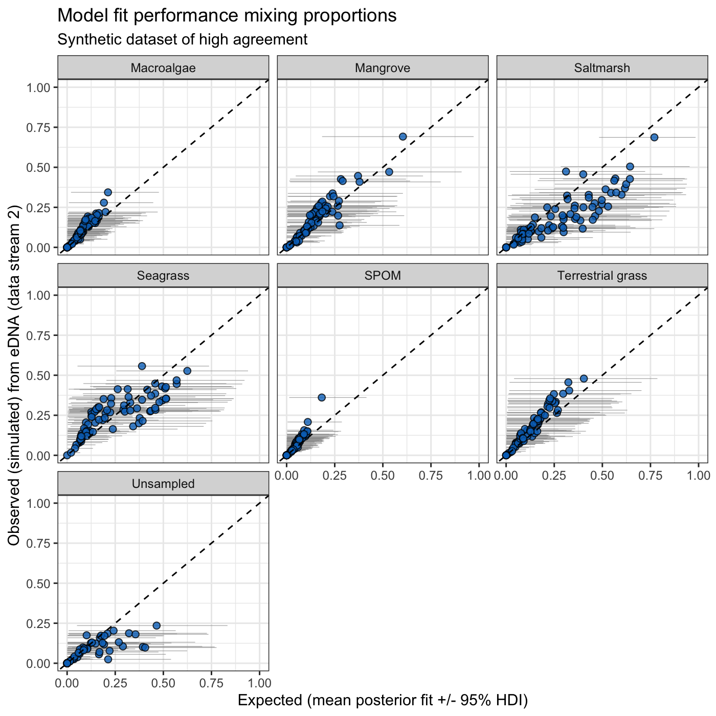
This plot compares observed vs. predicted mixing proportions for data stream 2, helping you assess how well the model captures the underlying signal. You can also explore how the model estimates compare to the stream 2 benchmark using Bayesian R2 (Gelman et al., 2019):
mixmustr_bayes_R2(
  model_fits[[1]]$model, summary = TRUE,
  data_streams_list = synthetic_df_convergent, target = "df_stream_2",
  order_ref = tracer_parameters$mus$source
)
#>              Source mean 2.5%HDI 97.5%HDI
#> 1        Macroalgae 0.57    0.48     0.66
#> 2          Mangrove 0.61    0.52     0.70
#> 3         Saltmarsh 0.64    0.60     0.69
#> 4          Seagrass 0.61    0.57     0.66
#> 5              SPOM 0.53    0.40     0.67
#> 6 Terrestrial grass 0.59    0.49     0.68
#> 7         Unsampled 0.61    0.57     0.66
Recap: Using MixMustR
Here’s a quick summary of how to use MixMustR
effectively:
-
Prepare Input Data:
-
df_stream_1: Observed data (optionally with group labels) -
df_stream_2: Known mixing proportions (e.g., from eDNA)
-
-
Define Tracer Summaries:
-
mus: Mean tracer values per source -
sigmas: Standard deviation per tracer per source
-
-
Run Model Configurations:
- Use
run_mixmustr_models()with the default or custom configurations - Adjust Stan settings (iterations, chains, etc.) as needed
- Use
-
Visualize Results:
- Use
make_post_prop_long()and plotting functions to assess fit - Use
mixmustr_bayes_R2()to create a table of Bayesian R2 values
- Use
Optional: Custom Input Creation
If you want more control, you can use
mixmustr_wrangle_input() directly to prepare the Stan input
list. This is helpful if you’re modifying the Stan code or working
outside the wrapper functions.
References
- Stock, B. C., Semmens, B. X. (2016). MixSIAR GUI User Manual. https://github.com/brianstock/MixSIAR