General usage
howto.RmdOverview
This guideline provides a series of practical examples on how a user
might take advantage of the functionalities offered by
ereefs. But first we need to load ereefs — if
you have not done so yet, please see our README page for
installation instructions:
The current package supports both curvilinear EMS files that provide
cell corners and regular regridded files that only provide cell centres.
The plotting functions detect the available geometry and reconstruct map
polygons from centre coordinates when needed. For scalar variables, the
default colour palette is now viridis.
What datasets are available?
The eReefs models have been run in multiple configurations, with different grid resolutions, forcing datasets, variables, output frequencies, and file formats. For the latest overview of open-access marine model results, including guidance on how to find current NCI-served eReefs outputs and what is included in the different products, start with the eReefs open-access dataset page: Marine model results.
Once you have found a candidate NetCDF file or THREDDS catalog,
inspect_ereefs_data() can give you a quick R-side summary
of the available variables, dimensions, spatial coverage, and date
coverage before you request a large extraction.
Inspecting available data
Before extracting data from an unfamiliar NetCDF file or THREDDS
catalog, use inspect_ereefs_data() to see what is
available. It reads metadata, coordinates, and time information rather
than full model variable arrays, so it is a safe first step for large
OPeNDAP-served files:
library(ereefs)

inspection <- inspect_ereefs_data(
  "../notebooks/demo_data/regular_demo_2020-01.nc"
)

inspection$summary
## # A tibble: 1 × 19
## requested_input inspected_source source_type file_count file_start file_end
## <chr> <chr> <chr> <int> <date> <date>
## 1 ../notebooks/de… ../notebooks/de… netcdf 1 2020-01-01 2020-01-01
## # ℹ 13 more variables: time_start <dttm>, time_end <dttm>, time_step <chr>,
## # longitude_min <dbl>, longitude_max <dbl>, latitude_min <dbl>,
## # latitude_max <dbl>, grid_type <chr>, i_count <int>, j_count <int>,
## # k_count <int>, variable_count <int>, data_variable_count <int>
inspection$variables## # A tibble: 14 × 8
## variable units long_name standard_name dimensions dimension_roles
## <chr> <chr> <chr> <chr> <chr> <chr>
## 1 botz m Depth of… depth i,j i,j
## 2 eta m Surface … sea_surface_… i,j,time i,j,time
## 3 salt PSU salinity NA i,j,k,time i,j,k,time
## 4 temp degC temperat… NA i,j,k,time i,j,k,time
## 5 u m s-1 Eastward… eastward_sea… i,j,k,time i,j,k,time
## 6 v m s-1 Northwar… northward_se… i,j,k,time i,j,k,time
## 7 i NA i NA i i
## 8 j NA j NA j j
## 9 k NA k NA k k
## 10 k_grid NA k_grid NA k_grid k
## 11 latitude degrees_north NA NA j j
## 12 longitude degrees_east NA NA i i
## 13 time days since 2020… time NA time time
## 14 z_grid m NA NA k_grid k
## # ℹ 2 more variables: n_dimensions <int>, is_data_variable <lgl>The summary table reports spatial coverage, time
coverage, grid style, grid dimensions, and variable counts. The
variables table lists variable names, units, long names,
standard names, dimensions, dimension roles, and whether each row
appears to be a model data variable rather than a coordinate or grid
variable. For THREDDS catalogs, inspection$files also lists
the catalog files used to infer file-level date coverage.
Making maps and animations from eReefs output
Static maps
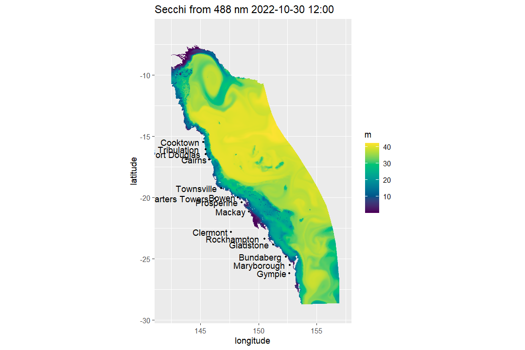
One can create a map of a scalar field such as Secchi depth from a live NCI simple-format file:
map_ereefs(
  var_name = "Secchi", target_date = as.Date("2022-10-30"),
  input_file = "https://thredds.nci.org.au/thredds/dodsC/fx3/gbr4_H4p0_ABARRAr2_OBRAN2020_FG2Gv3_B4p2_Cq5b_Dhnd/gbr4_H4p0_ABARRAr2_OBRAN2020_FG2G_B4p2_Cq5b_Dhnd_simple_2022-10-30.nc"
)
If you would prefer a smoother-looking presentation figure,
map_ereefs() can optionally rasterise the polygons to a
regular display grid and interpolate between the display pixels. This
only affects how the map is drawn; it does not change the extracted
values:
map_ereefs(
  var_name = "Secchi", target_date = as.Date("2022-10-30"),
  input_file = "https://thredds.nci.org.au/thredds/dodsC/fx3/gbr4_H4p0_ABARRAr2_OBRAN2020_FG2Gv3_B4p2_Cq5b_Dhnd/gbr4_H4p0_ABARRAr2_OBRAN2020_FG2G_B4p2_Cq5b_Dhnd_simple_2022-10-30.nc",
  plot_style = "smooth",
  smooth_pixels = 900
)
The same plotting path also works on regular-grid products that only provide cell centres. For example, here is a monthly mean surface temperature map from the AIMS regular-grid THREDDS catalog:
map_ereefs(
  var_name = "temp_mean", target_date = as.Date("2019-10-01"),
  input_file = "https://thredds.ereefs.aims.gov.au/thredds/catalog/ereefs/gbr1_2.0/stats-monthly-monthly/catalog.xml",
  box_bounds = c(149.2, 150.9, -20.4, -19.4)
)
The colour scale and display style can still be customised explicitly:
map_ereefs(
  var_name = "temp_mean", target_date = as.Date("2019-10-01"),
  input_file = "https://thredds.ereefs.aims.gov.au/thredds/catalog/ereefs/gbr1_2.0/stats-monthly-monthly/catalog.xml",
  box_bounds = c(149.2, 150.9, -20.4, -19.4),
  scale_lim = c(24, 27), plot_style = "smooth", smooth_pixels = 700
)
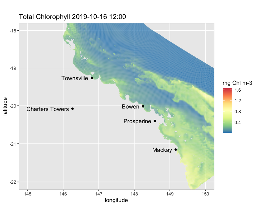
We can also plot different variables such as ammonium at a particular depth (e.g., 5 m below MSL; default is at the surface), add a land map to the plot, and focus on a particular region:
map_ereefs(
  var_name = "NH4", target_date = as.Date("2022-10-30"),
  layer = -5,
  input_file = "https://thredds.nci.org.au/thredds/dodsC/fx3/gbr4_H4p0_ABARRAr2_OBRAN2020_FG2Gv3_B4p2_Cq5b_Dhnd/gbr4_H4p0_ABARRAr2_OBRAN2020_FG2G_B4p2_Cq5b_Dhnd_simple_2022-10-30.nc",
  land_map = TRUE, box_bounds = c(145, 150, -22, -18), scale_lim = c(0, 2.5)
)
Animations
map_ereefs_movie() now assembles GIF or MP4 animations
directly. Numeric variables use one shared colour scale across all
frames by default, so the colours remain comparable from one time-step
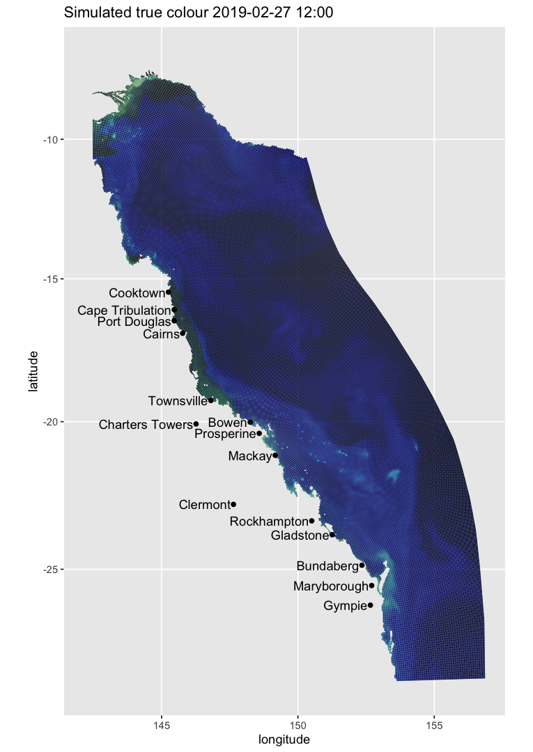
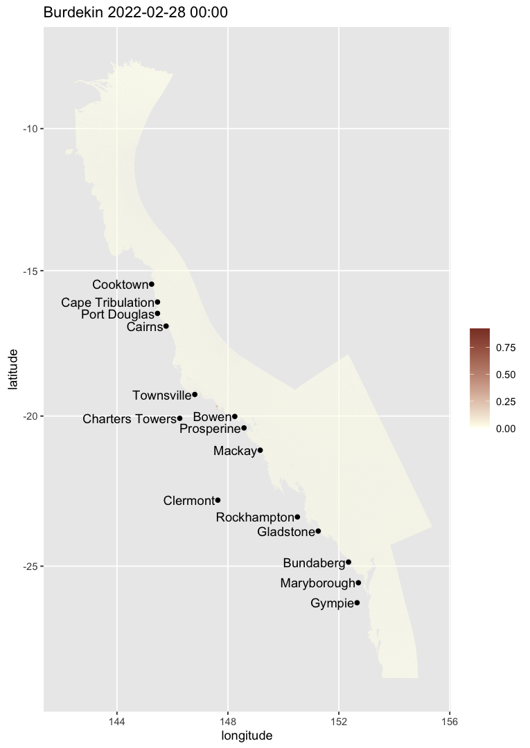
to the next. The example below creates a short true-colour GIF near the
mouth of the Burdekin River over a few days in February 2019. Temporary
frame images are removed after the GIF is created unless
keep_frames = TRUE:
# code not run
burdekin_movie <- map_ereefs_movie(
  var_name = "true_colour",
  start_date = as.Date("2019-02-01"),
  end_date = as.Date("2019-02-05"),
  input_file = "https://thredds.nci.org.au/thredds/catalog/fx3/gbr4_H4p0_ABARRAr2_OBRAN2020_FG2Gv3_B4p2_Cq5b_Dhnd/catalog.xml",
  layer = "surface",
  land_map = TRUE,
  box_bounds = c(147.0, 148.3, -20.1, -19.0),
  output_dir = "vignettes/burdekin_animation_frames",
  animation_format = "gif",
  animation_file = "vignettes/vignette-fig-burdekin-true-colour-animation.gif",
  fps = 2
)
Plotting vertical profiles and slices through the data
The code example below extracts the data from a vertical slice of
ammonium along a short transect extending about 60 km offshore from
Townsville using live OPeNDAP data from the NCI simple file. A slice can
also be defined along a long, curvy line, for example a boat track, by
passing a multi-row data frame of latitude and longitude points to
geolocation in get_ereefs_slice(). One can
also get data from multiple variables by making var_names a
vector (e.g., var_names = c("temp", "salt")).
temp_slice <- get_ereefs_slice(
  var_names = "NH4",
  target_date = as.POSIXct("2022-10-30 12:00:00", tz = "Etc/GMT-10"),
  geolocation = data.frame(latitude = c(-19.26639219, -19.26639219), longitude = c(146.805701, 147.38)),
  input_file = "https://thredds.nci.org.au/thredds/catalog/fx3/gbr4_H4p0_ABARRAr2_OBRAN2020_FG2Gv3_B4p2_Cq5b_Dhnd/catalog.xml"
)
Now visualise the results:
plot_ereefs_slice(temp_slice, var_name = "NH4", scale_col = "viridis", var_units = "mg N m-3")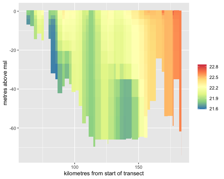
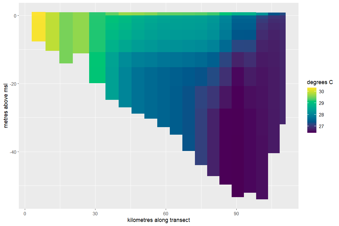
The same multi-point geolocation interface can be used
to define a curved or zig-zag transect. Here is a live OPeNDAP example
using hydrodynamic temperature data from an arc-shaped transect that
bends north-east away from Townsville:
arc_transect <- data.frame(
  latitude = c(-19.26639219, -19.18, -19.02, -18.84, -18.70),
  longitude = c(146.805701, 146.95, 147.12, 147.33, 147.56)
)

arc_slice <- get_ereefs_slice(
  var_names = "temp",
  target_date = as.POSIXct("2022-10-30 12:00:00", tz = "Etc/GMT-10"),
  geolocation = arc_transect,
  input_file = "https://thredds.nci.org.au/thredds/dodsC/fx3/gbr4_H4p0_ABARRAr2_OBRAN2020_FG2Gv3_Dhnd/gbr4_simple_2022-10-30.nc"
)
We can map the surface temperature field from the same dataset, then overlay the curved transect path:
library(ggplot2)

arc_map <- map_ereefs(
  var_name = "temp",
  target_date = as.POSIXct("2022-10-30 12:00:00", tz = "Etc/GMT-10"),
  layer = "surface",
  input_file = "https://thredds.nci.org.au/thredds/dodsC/fx3/gbr4_H4p0_ABARRAr2_OBRAN2020_FG2Gv3_Dhnd/gbr4_simple_2022-10-30.nc",
  box_bounds = c(146.6, 147.8, -19.5, -18.5)
) +
  geom_path(
    data = arc_transect,
    aes(x = longitude, y = latitude),
    inherit.aes = FALSE,
    colour = "black",
    linewidth = 1.6,
    lineend = "round"
  )

arc_map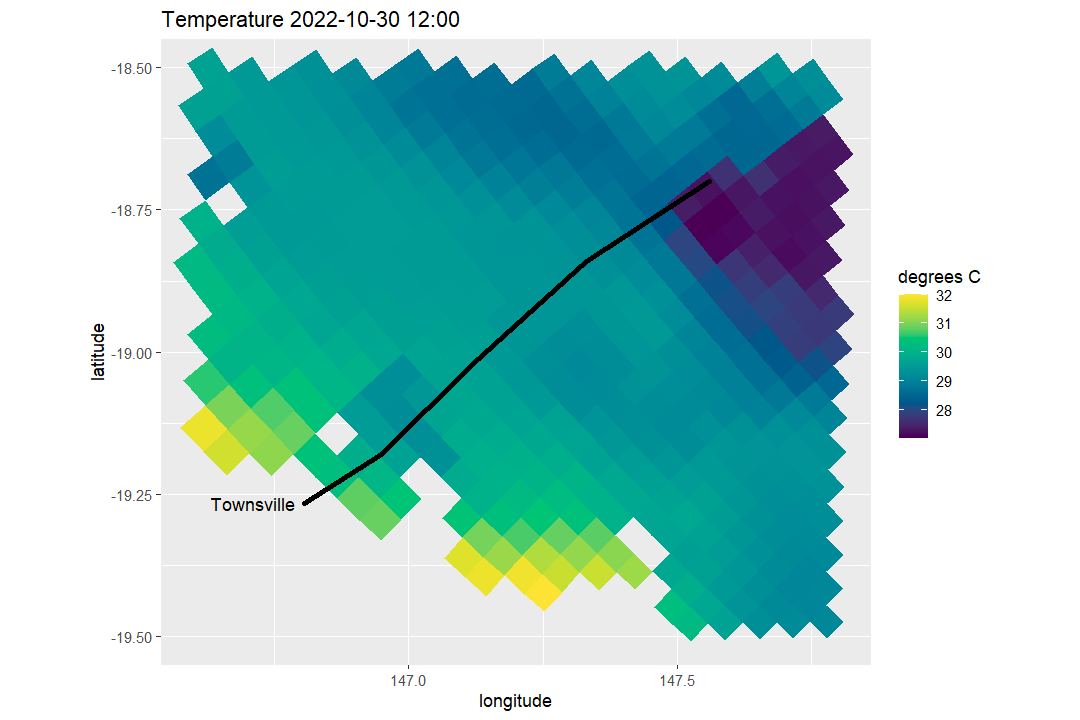
Then we can visualise the corresponding vertical slice:
plot_ereefs_slice(
  arc_slice,
  var_name = "temp",
  scale_col = "viridis",
  var_units = "degrees C"
)
We can also extract a vertical profile (rather than a slice) at a single location and time from the same live OPeNDAP file:
profile_data <- get_ereefs_profile(
  var_names = "NH4",
  start_date = as.POSIXct("2022-10-30 12:00:00", tz = "Etc/GMT-10"),
  end_date = as.POSIXct("2022-10-30 12:00:00", tz = "Etc/GMT-10"),
  geolocation = c(-19.5, 148.0),
  input_file = "https://thredds.nci.org.au/thredds/dodsC/fx3/gbr4_H4p0_ABARRAr2_OBRAN2020_FG2Gv3_B4p2_Cq5b_Dhnd/gbr4_H4p0_ABARRAr2_OBRAN2020_FG2G_B4p2_Cq5b_Dhnd_simple_2022-10-30.nc"
)
Now visualise the results:
plot_ereefs_profile(
  profile_data, var_name = "NH4", target_date = as.POSIXct("2022-10-30 12:00:00", tz = "Etc/GMT-10")
)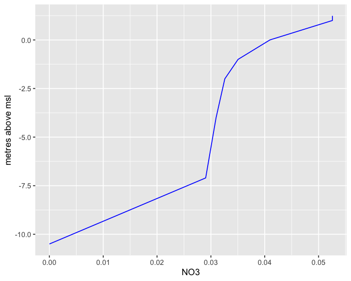
get_ereefs_profile() now favours robustness over
low-level NetCDF slicing, which makes it slower for long requests but
much less brittle for OPeNDAP-served data.
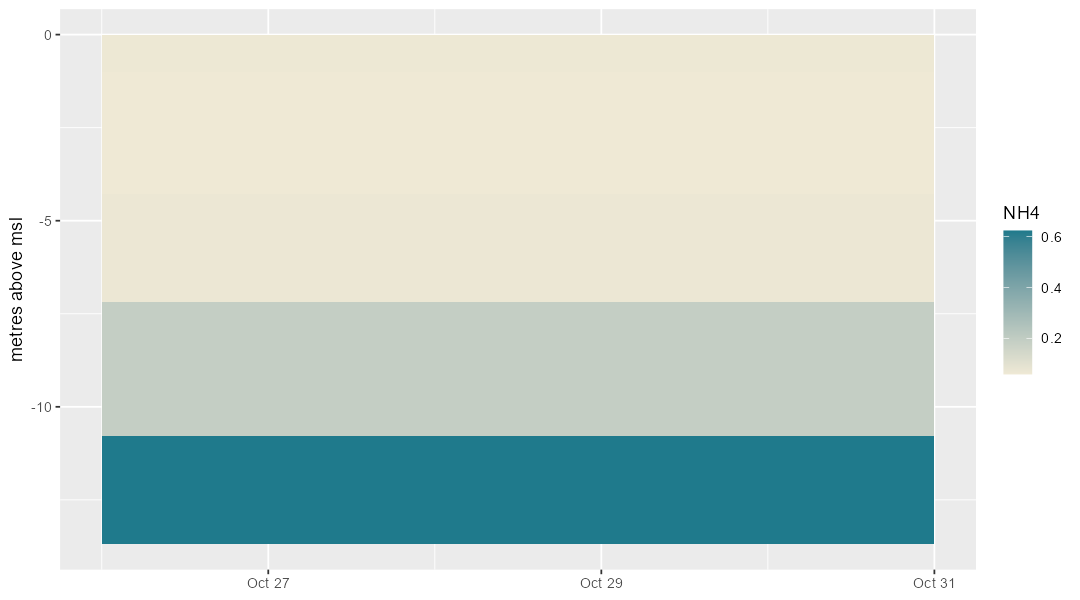
It can also extract a sequence of profiles over a date range. The
next example uses the same live NCI catalog as the slice example above,
extracting NH4 for five daily simple files at a point
half-way along the Townsville transect:
profile_range <- get_ereefs_profile(
  var_names = "NH4",
  start_date = as.POSIXct("2022-10-26 12:00:00", tz = "Etc/GMT-10"),
  end_date = as.POSIXct("2022-10-30 12:00:00", tz = "Etc/GMT-10"),
  geolocation = c(-19.26639219, 147.0928505),
  input_file = "https://thredds.nci.org.au/thredds/catalog/fx3/gbr4_H4p0_ABARRAr2_OBRAN2020_FG2Gv3_B4p2_Cq5b_Dhnd/catalog.xml"
)
plot_ereefs_zvt() shows the resulting profile sequence
as a time-depth plot:
plot_ereefs_zvt(
  profile_range,
  var_name = "NH4",
  scale_col = c("#efe9d5", "#1f7a8c")
)
Time series
We can also extract a time-series of surface data at a single or multiple specified locations (choose menu option 11):
tsdata <- get_ereefs_ts(
  var_names = c("temp", "salt"),
  start_date = as.POSIXct("2020-01-01 00:00:00", tz = "Etc/GMT-10"),
  end_date = as.POSIXct("2020-01-03 00:00:00", tz = "Etc/GMT-10"),
  geocoordinates = data.frame(latitude = -19.75, longitude = 146.75),
  input_file = "notebooks/demo_data/regular_demo_2020-01.nc"
)
The returned object is a tibble, with NetCDF variable metadata attached as attributes. This keeps the table itself tidy while still making units and longer variable descriptions available for plotting labels or reporting:
For example, we can quickly plot the extracted surface temperature and salinity time-series:
library(ggplot2)

ggplot(tsdata, aes(x = time)) +
  geom_line(aes(y = temp, colour = "temp")) +
  geom_point(aes(y = temp, colour = "temp")) +
  geom_line(aes(y = salt, colour = "salt")) +
  geom_point(aes(y = salt, colour = "salt")) +
  labs(x = NULL, y = "value", colour = "variable")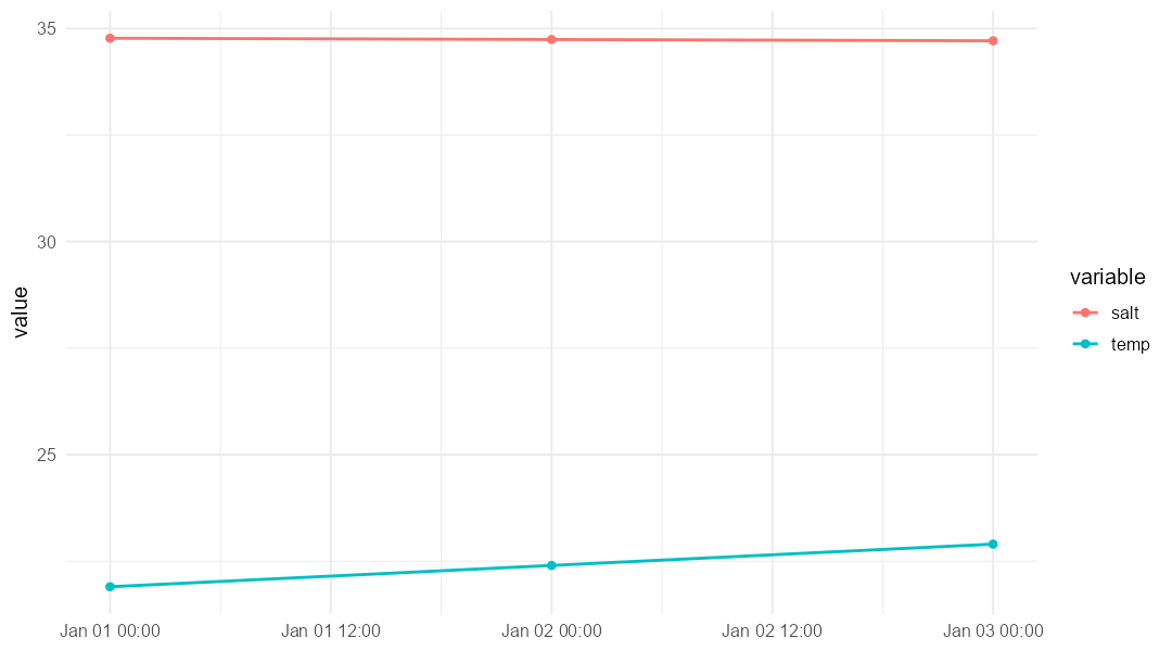
When input_file is a THREDDS catalog rather than a
single NetCDF file, the package now works out which files are needed to
cover the requested period. If the requested period extends beyond what
is currently present in that catalog, the available part is returned
with a warning.
The locations could even be at all the Marine Monitoring Program routine water quality sampling locations:
mmpdata <- get_ereefs_ts(
  var_names = c("salt", "TN"), geocoordinates = "mmp",
  start_date = c(2018, 1, 1), end_date = c(2018, 2, 28)
)
The time-series can also be extract at a specified depth of 5 m below MSL:
deeperdata <- get_ereefs_ts(
  var_names = "temp", geocoordinates = c(-19.75, 146.75),
  start_date = as.POSIXct("2020-01-01 00:00:00", tz = "Etc/GMT-10"),
  end_date = as.POSIXct("2020-01-03 00:00:00", tz = "Etc/GMT-10"),
  layer = -5,
  input_file = "notebooks/demo_data/regular_demo_2020-01.nc"
)
For depth-resolved variables, layer = "surface" now
refers to the shallowest wet model layer at each output time, while
layer = "bottom" refers to the deepest wet layer. This is
more robust in tidally shallow cells where the largest k
index can occasionally be dry.
One could also have set the argument layer = "bottom" to
extract a time-series of data at the bottom of the water column.
However, to extract a time-series of data averaged over the depth of the
water column, the user woul use the function
get_ereefs_depth_integrated_ts:
intdata <- get_ereefs_depth_integrated_ts(
  var_names = "temp", geocoordinates = c(-19.75, 146.75),
  start_date = as.POSIXct("2020-01-01 00:00:00", tz = "Etc/GMT-10"),
  end_date = as.POSIXct("2020-01-03 00:00:00", tz = "Etc/GMT-10"),
  input_file = "notebooks/demo_data/regular_demo_2020-01.nc"
)
Other options include extracting a time-series of the mass per square metre of a variable, integrated over the depth of the water column:
intdatapermass <- get_ereefs_depth_integrated_ts(
  var_names = "temp", geocoordinates = c(-19.75, 146.75),
  start_date = as.POSIXct("2020-01-01 00:00:00", tz = "Etc/GMT-10"),
  end_date = as.POSIXct("2020-01-03 00:00:00", tz = "Etc/GMT-10"),
  input_file = "notebooks/demo_data/regular_demo_2020-01.nc", mass = TRUE
)
or extracting a time-series of data at a specified depth below the tidal free surface (rather than below MSL):
tidalintdata <- get_ereefs_depth_specified_ts(
  var_names = "temp", geocoordinates = c(-19.75, 146.75),
  start_date = as.POSIXct("2020-01-01 00:00:00", tz = "Etc/GMT-10"),
  end_date = as.POSIXct("2020-01-03 00:00:00", tz = "Etc/GMT-10"),
  input_file = "notebooks/demo_data/regular_demo_2020-01.nc", depth = 2.0
)
Those depth-aware series can also be compared visually:
depth_plot_data <- rbind(
  data.frame(time = deeperdata$time, value = deeperdata$temp, series = "5 m below MSL"),
  data.frame(time = intdata$time, value = intdata$temp, series = "depth average"),
  data.frame(time = tidalintdata$time, value = tidalintdata$temp, series = "2 m below free surface")
)

ggplot(depth_plot_data, aes(x = time, y = value, colour = series)) +
  geom_line() +
  geom_point() +
  labs(x = NULL, y = "temperature")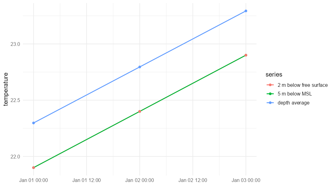
If eta is not available in a selected simple-format
file, get_ereefs_depth_specified_ts() now warns and assumes
eta = 0 instead of stopping. That keeps centre-only simple
files usable while making the approximation explicit.
If z_grid is absent but zc is present in a
simple-format file, the package now reconstructs layer interfaces from
zc using midpoint assumptions and resets the top interface
to 1e20 to match the standard EMS convention.
If a single requested timestamp does not exactly match a model output time, the package now falls back to the nearest available time and warns so the substitution is explicit.