library(RNetCDF) # working with netcdf files (incl. via OPeNDAP)
library(raster) # creating and manipuling rastersAccessing eReefs data from the AIMS eReefs THREDDS server
Basic access with OPeNDAP
Learn the basics of extracting eReefs data from the AIMS eReefs THREDDS server with OPeNDAP in .
In this tutorial we will look at how to access eReefs data directly from the AIMS eReefs THREDDS server in R.
This server hosts aggregated eReefs model data in NetCDF file format and offers access to the data files via OPeNDAP, HTTP Server, and Web Map Service (WMS). While we could download the data files manually via the HTTPServer link, this approach is cumbersome when downloading multiple files, given their large size. Thankfully, OPeNDAP provides a way to access the data files over the internet and extract only the data we want.
For example, say we want the daily mean surface temperature at a single location for the last 30 days. If we were to download the 30 individual daily aggregated NetCDF files, with each file ~ 350 Mb, this would require us to download over 10 Gb of data just to get 300 numbers. The vast majority of this data would be irrelevant to our needs as the NetCDF files contain data for a range of variables, at a range of depths, for many, many locations. However, with OPeNDAP, we can extract the daily mean values directly from the server without downloading any unneeded data.
Motivating problem
We will extract the daily mean water temperature for the 10th of October 2022 at 1.5 m depth across the entire scope of the eReefs model. We will then save and plot this data. This example will introduce the basics of how to connect to files on the server and extract the data we want.
R packages
While the ncdf4 package is commonly used to work with NetCDF files in R, it does not offer compatibility with OPeNDAP for Windows (only Mac and Linux). For this reason we will use the RNetCDF package which offers similar functionality and Windows compatibility with OPeNDAP. Note that if you are using Mac or Linux and wish to use ncdf4, the functions used herein have obvious analogues; for example ncdf4::nc_open() vs. RNetCDF::open.nc().
Connect to a file on the server
First we need to find the right NetCDF file on the server. The available eReefs data NetCDF files are listed in the AIMS eReefs THREDDS catalogue. We will navigate to the eReefs 4 km Hydrodynamic Model daily aggregated data for the month of October 2022 and copy the OPeNDAP data URL.
input_file <- "https://thredds.ereefs.aims.gov.au/thredds/dodsC/ereefs/gbr4_v4/daily-monthly/EREEFS_AIMS-CSIRO_gbr4_v4_hydro_daily-monthly-2022-10.nc"We can then open a connection to this file using the RNetCDF::open.nc function.
dailyAggOct22.nc <- open.nc(input_file)If you wish to download NetCDF files from the server you can click the HTTPServer link instead of OPeNDAP. The file can then be loaded into R by specifying the path: open.nc("<path to downloaded file>").
Print a file summary
If we wish to investigate the structure of the file we have connected to, including what variables and dimensions are available, we can print a summary.
summary <- print.nc(dailyAggOct22.nc)
summary
netcdf classic {
dimensions:
    time = UNLIMITED ; // (31 currently)
    k = 17 ;
    latitude = 723 ;
    longitude = 491 ;
variables:
    NC_FLOAT mean_cur(longitude, latitude, k, time) ;
        NC_CHAR mean_cur:puv__parameter = "http://vocab.nerc.ac.uk/collection/P01/current/LCEWMP01/" ;
        NC_CHAR mean_cur:coordinates = "time zc latitude longitude" ;
        NC_CHAR mean_cur:units = "ms-1" ;
        NC_CHAR mean_cur:short_name = "mean_cur" ;
        NC_CHAR mean_cur:aggregation = "mean_speed" ;
        NC_CHAR mean_cur:standard_name = "mean_current_speed" ;
        NC_CHAR mean_cur:long_name = "mean_current_speed" ;
        NC_INT mean_cur:_ChunkSizes = 1, 1, 133, 491 ;
    NC_FLOAT salt(longitude, latitude, k, time) ;
        NC_CHAR salt:puv__parameter = "http://vocab.nerc.ac.uk/collection/P01/current/PSLTMP01/" ;
        NC_CHAR salt:puv__uom = "http://qudt.org/vocab/unit/PSU" ;
        NC_CHAR salt:coordinates = "time zc latitude longitude" ;
        NC_CHAR salt:short_name = "salt" ;
        NC_CHAR salt:aggregation = "Daily" ;
        NC_CHAR salt:units = "PSU" ;
        NC_CHAR salt:long_name = "Salinity" ;
        NC_INT salt:_ChunkSizes = 1, 1, 133, 491 ;
    NC_FLOAT temp(longitude, latitude, k, time) ;
        NC_CHAR temp:puv__parameter = "http://vocab.nerc.ac.uk/collection/P01/current/TEMPMP01/" ;
        NC_CHAR temp:coordinates = "time zc latitude longitude" ;
        NC_CHAR temp:short_name = "temp" ;
        NC_CHAR temp:aggregation = "Daily" ;
        NC_CHAR temp:units = "degrees C" ;
        NC_CHAR temp:long_name = "Temperature" ;
        NC_INT temp:_ChunkSizes = 1, 1, 133, 491 ;
    NC_FLOAT u(longitude, latitude, k, time) ;
        NC_CHAR u:vector_components = "u v" ;
        NC_CHAR u:puv__parameter = "http://vocab.nerc.ac.uk/collection/P01/current/LCEWMP01/" ;
        NC_CHAR u:coordinates = "time zc latitude longitude" ;
        NC_CHAR u:short_name = "u" ;
        NC_CHAR u:standard_name = "eastward_sea_water_velocity" ;
        NC_CHAR u:vector_name = "Currents" ;
        NC_CHAR u:aggregation = "Daily" ;
        NC_CHAR u:units = "ms-1" ;
        NC_CHAR u:long_name = "Eastward current" ;
        NC_INT u:_ChunkSizes = 1, 1, 133, 491 ;
    NC_FLOAT v(longitude, latitude, k, time) ;
        NC_CHAR v:vector_components = "u v" ;
        NC_CHAR v:puv__parameter = "http://vocab.nerc.ac.uk/collection/P01/current/LCNSMP01/" ;
        NC_CHAR v:coordinates = "time zc latitude longitude" ;
        NC_CHAR v:short_name = "v" ;
        NC_CHAR v:standard_name = "northward_sea_water_velocity" ;
        NC_CHAR v:vector_name = "Currents" ;
        NC_CHAR v:aggregation = "Daily" ;
        NC_CHAR v:units = "ms-1" ;
        NC_CHAR v:long_name = "Northward current" ;
        NC_INT v:_ChunkSizes = 1, 1, 133, 491 ;
    NC_DOUBLE zc(k) ;
        NC_CHAR zc:puv__uom = "http://vocab.nerc.ac.uk/collection/P06/current/ULAA/" ;
        NC_CHAR zc:units = "m" ;
        NC_CHAR zc:positive = "up" ;
        NC_CHAR zc:long_name = "Z coordinate" ;
        NC_CHAR zc:axis = "Z" ;
        NC_CHAR zc:coordinate_type = "Z" ;
        NC_CHAR zc:_CoordinateAxisType = "Height" ;
        NC_CHAR zc:_CoordinateZisPositive = "up" ;
    NC_DOUBLE time(time) ;
        NC_CHAR time:units = "days since 1990-01-01 00:00:00 +10" ;
        NC_CHAR time:long_name = "Time" ;
        NC_CHAR time:standard_name = "time" ;
        NC_CHAR time:coordinate_type = "time" ;
        NC_CHAR time:puv__uom = "http://vocab.nerc.ac.uk/collection/P06/current/UTAA/" ;
        NC_CHAR time:calendar = "gregorian" ;
        NC_CHAR time:_CoordinateAxisType = "Time" ;
        NC_INT time:_ChunkSizes = 1024 ;
    NC_DOUBLE latitude(latitude) ;
        NC_CHAR latitude:puv__uom = "http://vocab.nerc.ac.uk/collection/P06/current/DEGN/" ;
        NC_CHAR latitude:units = "degrees_north" ;
        NC_CHAR latitude:long_name = "Latitude" ;
        NC_CHAR latitude:standard_name = "latitude" ;
        NC_CHAR latitude:coordinate_type = "latitude" ;
        NC_CHAR latitude:projection = "geographic" ;
        NC_CHAR latitude:_CoordinateAxisType = "Lat" ;
    NC_DOUBLE longitude(longitude) ;
        NC_CHAR longitude:puv__uom = "http://vocab.nerc.ac.uk/collection/P06/current/DEGE/" ;
        NC_CHAR longitude:units = "degrees_east" ;
        NC_CHAR longitude:long_name = "Longitude" ;
        NC_CHAR longitude:standard_name = "longitude" ;
        NC_CHAR longitude:coordinate_type = "longitude" ;
        NC_CHAR longitude:projection = "geographic" ;
        NC_CHAR longitude:_CoordinateAxisType = "Lon" ;
    NC_FLOAT mean_wspeed(longitude, latitude, time) ;
        NC_CHAR mean_wspeed:puv__parameter = "http://vocab.nerc.ac.uk/collection/P01/current/ESEWMPXX/" ;
        NC_CHAR mean_wspeed:coordinates = "time latitude longitude" ;
        NC_CHAR mean_wspeed:units = "ms-1" ;
        NC_CHAR mean_wspeed:short_name = "mean_wspeed" ;
        NC_CHAR mean_wspeed:aggregation = "mean_speed" ;
        NC_CHAR mean_wspeed:standard_name = "mean_wind_speed" ;
        NC_CHAR mean_wspeed:long_name = "mean_wind_speed" ;
        NC_INT mean_wspeed:_ChunkSizes = 1, 133, 491 ;
    NC_FLOAT eta(longitude, latitude, time) ;
        NC_CHAR eta:puv__parameter = "http://vocab.nerc.ac.uk/collection/P01/current/ASLVMP01/" ;
        NC_CHAR eta:coordinates = "time latitude longitude" ;
        NC_CHAR eta:short_name = "eta" ;
        NC_CHAR eta:standard_name = "sea_surface_height_above_geoid" ;
        NC_CHAR eta:aggregation = "Daily" ;
        NC_CHAR eta:units = "metre" ;
        NC_CHAR eta:positive = "up" ;
        NC_CHAR eta:long_name = "Surface elevation" ;
        NC_INT eta:_ChunkSizes = 1, 133, 491 ;
    NC_FLOAT wspeed_u(longitude, latitude, time) ;
        NC_CHAR wspeed_u:puv__parameter = "http://vocab.nerc.ac.uk/collection/P01/current/ESEWMPXX/" ;
        NC_CHAR wspeed_u:vector_components = "wspeed_u wspeed_v" ;
        NC_CHAR wspeed_u:coordinates = "time latitude longitude" ;
        NC_CHAR wspeed_u:short_name = "wspeed_u" ;
        NC_CHAR wspeed_u:standard_name = "eastward_wind" ;
        NC_CHAR wspeed_u:vector_name = "Wind" ;
        NC_CHAR wspeed_u:aggregation = "Daily" ;
        NC_CHAR wspeed_u:units = "ms-1" ;
        NC_CHAR wspeed_u:long_name = "Eastward wind" ;
        NC_INT wspeed_u:_ChunkSizes = 1, 133, 491 ;
    NC_FLOAT wspeed_v(longitude, latitude, time) ;
        NC_CHAR wspeed_v:puv__parameter = "http://vocab.nerc.ac.uk/collection/P01/current/ESNSMPXX/" ;
        NC_CHAR wspeed_v:vector_components = "wspeed_u wspeed_v" ;
        NC_CHAR wspeed_v:coordinates = "time latitude longitude" ;
        NC_CHAR wspeed_v:short_name = "wspeed_v" ;
        NC_CHAR wspeed_v:standard_name = "northward_wind" ;
        NC_CHAR wspeed_v:vector_name = "Wind" ;
        NC_CHAR wspeed_v:aggregation = "Daily" ;
        NC_CHAR wspeed_v:units = "ms-1" ;
        NC_CHAR wspeed_v:long_name = "Northward wind" ;
        NC_INT wspeed_v:_ChunkSizes = 1, 133, 491 ;

// global attributes:
        NC_CHAR :Conventions = "CF-1.0" ;
        NC_CHAR :Parameter_File_Revision = "$Revision$" ;
        NC_CHAR :Run_ID = "4.0" ;
        NC_CHAR :Run_code = "SHOC grid|G3.00|H4.0|S-3.00|B0.00" ;
        NC_CHAR :_CoordSysBuilder = "ucar.nc2.dataset.conv.CF1Convention" ;
        NC_CHAR :aims_ncaggregate_buildDate = "2025-06-13T15:26:28+10:00" ;
        NC_CHAR :aims_ncaggregate_datasetId = "products__ncaggregate__ereefs__gbr4_v4__daily-monthly/EREEFS_AIMS-CSIRO_gbr4_v4_hydro_daily-monthly-2022-10" ;
        NC_CHAR :aims_ncaggregate_firstDate = "2022-10-01T00:00:00+10:00" ;
        NC_CHAR :aims_ncaggregate_inputs = "[products__ncaggregate__ereefs__gbr4_v4__raw/EREEFS_AIMS-CSIRO_gbr4_v4_hydro_raw_2022-10::MD5:be53ddf69130a8e39363f68ec599936b]" ;
        NC_CHAR :aims_ncaggregate_lastDate = "2022-10-31T00:00:00+10:00" ;
        NC_CHAR :bald__isPrefixedBy = "prefix_list" ;
        NC_CHAR :date_created = "Mon Oct 21 15:22:31 2024" ;
        NC_CHAR :description = "Aggregation of raw hourly input data (from eReefs AIMS-CSIRO GBR4 Hydrodynamic v4 subset) to daily means. Also calculates mean magnitude of wind and ocean current speeds. Data is regridded from curvilinear (per input data) to rectilinear via inverse weighted distance from up to 4 closest cells." ;
        NC_CHAR :ems_version = "v1.4.0 rev(7365)" ;
        NC_CHAR :history = "2025-06-13T14:12:13+10:00: vendor: AIMS; processing: None summaries
2025-06-13T15:26:28+10:00: vendor: AIMS; processing: Daily summaries" ;
        NC_CHAR :metadata_link = "https://eatlas.org.au/data/uuid/350aed53-ae0f-436e-9866-d34db7f04d2e" ;
        NC_CHAR :paramfile = "/g/data/et4/projects/eReefs/gbr4_H4p0_ABARRAr2_OBRAN2020_FG2Gv3_Dhnd/tran/gbr4_H4p0_ABARRAr2_OBRAN2020_FG2Gv3.tran" ;
        NC_CHAR :paramhead = "eReefs GBR 4k grid, with Atmospheric forcing using BARRAr2, open Ocean forcing using BRAN2020, river Flows forcing using G2G and QDES SOURCE; Deployed as a hindcast. Hydro GBR4 parameter file 4.0." ;
        NC_CHAR :prefix_list_puv__ = "https://w3id.org/env/puv#" ;
        NC_CHAR :technical_guide_link = "https://nextcloud.eatlas.org.au/apps/sharealias/a/aims-ereefs-platform-technical-guide-to-derived-products-from-csiro-ereefs-models-pdf" ;
        NC_CHAR :technical_guide_publish_date = "2020-08-18" ;
        NC_CHAR :title = "eReefs AIMS-CSIRO GBR4 Hydrodynamic v4 daily aggregation" ;
        NC_CHAR :DODS_EXTRA.Unlimited_Dimension = "time" ;
}
Extract data
Now that we have an open connection to a file on the server we need to extract the daily mean temperature at 1.5m depth for the 10th of October.
From the summary output above we can see that the variable corresponding to temperature is: \(\texttt{ temp(longitude, latitude, k, time)}\).
The dimensions for temperature are in brackets. This means that there is a temperature value for every combination of longitude, latitude, depth (k) and time. We can now see why these NetCDF files are so large.
To extract data from the file we will use the function
RNetCDF::var.get.nc(ncfile, variable, start=NA, count=NA, ...)
We need to give the function:
ncfile: a NetCDF file connection; in our casedailyAggOct22.nc.variable: the name or id of the data variable we wish to extract; in our case"temp".start: a vector of indices of where to start getting data, one for each dimension of the variable. Since we have \(\texttt{temp(longitude, latitude, k, time)}\) we need to tell the function where to start getting data along each of the four dimensions.count: similar to start, but specifying the number of temperature values to extract along each dimension.
Let’s look at how to construct our start and count vectors.
The default values of start and count are NA, in which case all data for the given variable will be extracted.
Depth: Starting with depth is easy because we have a constant value of interest (1.5 m). The index k corresponds to different depths as shown in the table below, where we see that for the 4km models k=16 maps to a depth of 1.5 m.
Table of eReefs depths corresponding to index k
| Index k (R) | Index k (Python) | Hydrodynamic 1km model | Hydrodynamic & BioGeoChemical 4km models |
|---|---|---|---|
| 1 | 0 | -140.00 | -145.00 |
| 2 | 1 | -120.00 | -120.00 |
| 3 | 2 | -103.00 | -103.00 |
| 4 | 3 | -88.00 | -88.00 |
| 5 | 4 | -73.00 | -73.00 |
| 6 | 5 | -60.00 | -60.00 |
| 7 | 6 | -49.00 | -49.00 |
| 8 | 7 | -39.50 | -39.50 |
| 9 | 8 | -31.00 | -31.00 |
| 10 | 9 | -24.00 | -23.75 |
| 11 | 10 | -18.00 | -17.75 |
| 12 | 11 | -13.00 | -12.75 |
| 13 | 12 | -9.00 | -8.80 |
| 14 | 13 | -5.25 | -5.55 |
| 15 | 14 | -2.35 | -3.00 |
| 16 | 15 | -0.50 | -1.50 |
| 17 | 16 | NA | -0.50 |
Time: Since we have the daily aggregated data for October 2022, and are interested only in a single day (the 10th), time is also a constant value. From the summary output we can see we have 31 time indexes, these correspond to the day of the month, therefore we want time=10.
Longitude and latitude: We want temperatures for every available longitude and latitude so we can plot the data across the entire spatial range of the eReefs model. Therefore we want to start at index 1 and count for the entire length of latitude and longitude. To get the lengths we could note the values from the summary output, where we see \(\texttt{longitude = 491}\) and \(\texttt{latitude = 723}\). However we could also get the lengths programmatically.
lon <- var.get.nc(dailyAggOct22.nc, "longitude")
lat <- var.get.nc(dailyAggOct22.nc, "latitude")
data.frame(length(lon), length(lat))
length.lon. length.lat.
1 491 723Within the eReefs NetCDF files, the dimensions \(\texttt{longitude, latitude, k, time}\) have corresponding variables longitude, latitude, zc, time (see summary output). Note that we would extract the dimension \(\texttt{k}\) variable with var.get.nc(..., variable = "zc").
Now we are ready to construct our start and count vectors and extract the data.
# SETUP START AND COUNT VECTORS
# Recall the order of the dimensions: (lon, lat, k , time)
# We start at lon=1, lat=1, k=16, time=10 and get temps for
# every lon and lat while holding depth and time constant
lon_st <- 1
lat_st <- 1
depth_st <- 16  # index k = 16 --> depth = 1.5 m
time_st <- 10   # index time = 10 --> 10th day of month

lon_ct <- length(lon) # get temps for all lons and lats
lat_ct <- length(lat)
time_ct <- 1  # Hold time and depth constant
depth_ct <- 1

start_vector <- c(lon_st, lat_st, depth_st, time_st)
count_vector <- c(lon_ct, lat_ct, time_ct, depth_ct)

# EXTRACT DATA
temps_10Oct22_1p5m <- var.get.nc(
  ncfile = dailyAggOct22.nc,
  variable = "temp",
  start = start_vector,
  count = count_vector
)

# Get the size of our extracted data
dims <- dim(temps_10Oct22_1p5m)
data.frame(nrows = dims[1], ncols = dims[2])
nrows ncols
1 491 723Close file connection
Now that our extracted data is stored in memory, we should close the connection to the NetCDF file on the server.
close.nc(dailyAggOct22.nc)Save the data
Now that we have our extracted data we may wish to save it for future use. To do this we first convert the data from its current form as a matrix array into a raster, and then save the raster as a NetCDF file (GeoTIFF and other formats are also possible).
When converting extracted eReefs data to rasters we need to apply the transpose t() and flip() functions in order to get the correct orientation.
temps_raster <- temps_10Oct22_1p5m |>
  t() |>   # transpose temps matrix
  raster(  # create raster
    xmn = min(lon), xmx = max(lon),
    ymn = min(lat), ymx = max(lat),
    crs = CRS("+init=epsg:4326")
  ) |>
  flip(direction = 'y') # flip the raster
Warning in CPL_crs_from_input(x): GDAL Message 1: +init=epsg:XXXX syntax is
deprecated. It might return a CRS with a non-EPSG compliant axis order.temps_rasterclass : RasterLayer
dimensions : 723, 491, 354993 (nrow, ncol, ncell)
resolution : 0.0299389, 0.02995851 (x, y)
extent : 142.1688, 156.8688, -28.69602, -7.036022 (xmin, xmax, ymin, ymax)
crs : +proj=longlat +datum=WGS84 +no_defs
source : memory
names : layer
values : 20.24341, 29.92736 (min, max)In the code chunk above we used pipes |>. Pipes are very useful when passing a dataset through a sequence of functions. In the code above we take our extracted temps, transpose them, turn them into a raster, and then flip the raster. The final result is saved to temps_raster.
Now we have our raster (in the correct orientation), saving it is easy.
# Save the raster file in the /data subdirectory
# Note the '.nc' file extension since we are going to save as NetCDF
save_file <- "data/ereefsDailyMeanWaterTemperature_10Oct2022_Depth1p5m.nc"

writeRaster(
  x = temps_raster, # what to save
  filename = save_file, # where to save it
  format = "CDF", # what format to save it as
  overwrite = TRUE # whether to replace any existing file with the same name
)
The raster package uses the ncdf4 package to deal with NetCDF files. You can install this package by running install.packages("ncdf4") from an R console.
To prove to ourselves that this worked, lets read the file back in and plot it.
# Read back in the saved NetCDF file as a raster
saved_temps <- raster(save_file)

# Plot the data
plot(saved_temps)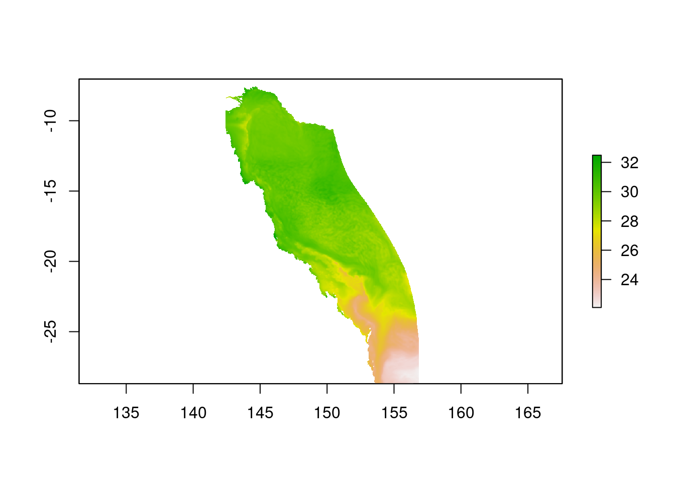
Hooray! We can now see our saved data plotted in Figure 1.