Plotting eReefs data

Times series plots

Learn how to create time series plots of eReefs data in python.

In this notebook we use OPeNDAP to extract time series data at a single location of interest, then plot this data. This extraction process can also be done with the AIMS eReefs data extraction tool. If you which to perform bigger extractions then we recommend using this tool instead of this process outlined in this example.

Note: This script has no error checking and so changing the date ranges or locations might result in out of bounds errors.

Load the required Python libraries

from netCDF4 import Dataset, num2date
import matplotlib.pyplot as plt
import cartopy
import cartopy.crs as ccrs
import os
import datetime
import pandas as pd
import numpy as np
cartopy.config['data_dir'] = os.getenv('CARTOPY_DIR', cartopy.config.get('data_dir'))

Choose OPeNDAP end point

The first part of the process is to choose the OPeNDAP end point on the AIMS eReefs THREDDS server. You can view the products in the AIMS eReefs THREDDS catalogue. At this stage there is no grouped OPeNDAP service for the entire time series and so this script only works for looking at a single month of data. Hopefully this can be improved in the future.

# Connect to the OpeNDAP endpoint for the specified month.
month = 3
year = 2020
netCDF_datestr = str(year)+'-'+format(month, '02')
print(netCDF_datestr)

2020-03

# OPeNDAP URL to file "EREEFS_AIMS-CSIRO_gbr4_v2_hydro_daily-monthly-YYYY-MM.nc". Hydrodynamic 4km model, daily data for the month specified
inputFile = "https://thredds.ereefs.aims.gov.au/thredds/dodsC/ereefs/gbr4_v2/daily-monthly/EREEFS_AIMS-CSIRO_gbr4_v2_hydro_daily-monthly-"+netCDF_datestr+".nc"

nc_data = Dataset(inputFile, 'r')
print(nc_data.title)

# To find a list of the variables uncomment the next line:
print(repr(nc_data.variables))

eReefs AIMS-CSIRO GBR4 Hydrodynamic v2 daily aggregation
{'mean_cur': <class 'netCDF4._netCDF4.Variable'>
float32 mean_cur(time, k, latitude, longitude)
    coordinates: time zc latitude longitude
    substanceOrTaxon_id: http://environment.data.gov.au/def/feature/ocean_current
    units: ms-1
    puv__parameter: http://vocab.nerc.ac.uk/collection/P01/current/LCEWMP01/
    medium_id: http://environment.data.gov.au/def/feature/ocean
    unit_id: http://qudt.org/vocab/unit#MeterPerSecond
    short_name: mean_cur
    aggregation: mean_speed
    standard_name: mean_current_speed
    long_name: mean_current_speed
    _ChunkSizes: [  1   1 133 491]
unlimited dimensions: time
current shape = (31, 17, 723, 491)
filling off, 'salt': <class 'netCDF4._netCDF4.Variable'>
float32 salt(time, k, latitude, longitude)
    qudt__unit: http://qudt.org/vocab/unit/PSU
    puv__parameter: http://vocab.nerc.ac.uk/collection/P01/current/PSLTMP01/
    coordinates: time zc latitude longitude
    substanceOrTaxon_id: http://sweet.jpl.nasa.gov/2.2/matrWater.owl#SaltWater
    scaledQuantityKind_id: http://environment.data.gov.au/def/property/practical_salinity
    short_name: salt
    aggregation: Daily
    units: PSU
    medium_id: http://environment.data.gov.au/def/feature/ocean
    unit_id: http://environment.data.gov.au/water/quality/def/unit/PSU
    long_name: Salinity
    _ChunkSizes: [  1   1 133 491]
unlimited dimensions: time
current shape = (31, 17, 723, 491)
filling off, 'temp': <class 'netCDF4._netCDF4.Variable'>
float32 temp(time, k, latitude, longitude)
    puv__parameter: https://vocab.nerc.ac.uk/collection/P01/current/TEMPMP01/
    coordinates: time zc latitude longitude
    substanceOrTaxon_id: http://sweet.jpl.nasa.gov/2.2/matrWater.owl#SaltWater
    scaledQuantityKind_id: http://environment.data.gov.au/def/property/sea_water_temperature
    short_name: temp
    aggregation: Daily
    units: degrees C
    medium_id: http://environment.data.gov.au/def/feature/ocean
    unit_id: http://qudt.org/vocab/unit#DegreeCelsius
    long_name: Temperature
    _ChunkSizes: [  1   1 133 491]
unlimited dimensions: time
current shape = (31, 17, 723, 491)
filling off, 'u': <class 'netCDF4._netCDF4.Variable'>
float32 u(time, k, latitude, longitude)
    vector_components: u v
    coordinates: time zc latitude longitude
    substanceOrTaxon_id: http://environment.data.gov.au/def/feature/ocean_current
    vector_name: Currents
    aggregation: Daily
    units: ms-1
    long_name: Eastward current
    puv__parameter: http://vocab.nerc.ac.uk/collection/P01/current/LCEWMP01/
    scaledQuantityKind_id: http://environment.data.gov.au/def/property/sea_water_velocity_eastward
    short_name: u
    standard_name: eastward_sea_water_velocity
    medium_id: http://environment.data.gov.au/def/feature/ocean
    unit_id: http://qudt.org/vocab/unit#MeterPerSecond
    _ChunkSizes: [  1   1 133 491]
unlimited dimensions: time
current shape = (31, 17, 723, 491)
filling off, 'v': <class 'netCDF4._netCDF4.Variable'>
float32 v(time, k, latitude, longitude)
    vector_components: u v
    coordinates: time zc latitude longitude
    substanceOrTaxon_id: http://environment.data.gov.au/def/feature/ocean_current
    vector_name: Currents
    aggregation: Daily
    units: ms-1
    long_name: Northward current
    puv__parameter: http://vocab.nerc.ac.uk/collection/P01/current/LCNSMP01/
    scaledQuantityKind_id: http://environment.data.gov.au/def/property/sea_water_velocity_northward
    short_name: v
    standard_name: northward_sea_water_velocity
    medium_id: http://environment.data.gov.au/def/feature/ocean
    unit_id: http://qudt.org/vocab/unit#MeterPerSecond
    _ChunkSizes: [  1   1 133 491]
unlimited dimensions: time
current shape = (31, 17, 723, 491)
filling off, 'zc': <class 'netCDF4._netCDF4.Variable'>
float64 zc(k)
    positive: up
    coordinate_type: Z
    units: m
    long_name: Z coordinate
    axis: Z
    _CoordinateAxisType: Height
    _CoordinateZisPositive: up
unlimited dimensions: 
current shape = (17,)
filling off, 'time': <class 'netCDF4._netCDF4.Variable'>
float64 time(time)
    units: days since 1990-01-01 00:00:00 +10
    long_name: Time
    standard_name: time
    coordinate_type: time
    puv__uom: http://vocab.nerc.ac.uk/collection/P06/current/UTAA/
    calendar: gregorian
    _CoordinateAxisType: Time
    _ChunkSizes: 1024
unlimited dimensions: time
current shape = (31,)
filling off, 'latitude': <class 'netCDF4._netCDF4.Variable'>
float64 latitude(latitude)
    long_name: Latitude
    standard_name: latitude
    units: degrees_north
    coordinate_type: latitude
    projection: geographic
    puv__ofProperty: http://vocab.nerc.ac.uk/collection/S06/current/S0600045/
    puv__uom: http://vocab.nerc.ac.uk/collection/P06/current/DEGN/
    _CoordinateAxisType: Lat
unlimited dimensions: 
current shape = (723,)
filling off, 'longitude': <class 'netCDF4._netCDF4.Variable'>
float64 longitude(longitude)
    standard_name: longitude
    long_name: Longitude
    units: degrees_east
    puv__uom: http://vocab.nerc.ac.uk/collection/P06/current/DEGE/
    coordinate_type: longitude
    projection: geographic
    _CoordinateAxisType: Lon
unlimited dimensions: 
current shape = (491,)
filling off, 'mean_wspeed': <class 'netCDF4._netCDF4.Variable'>
float32 mean_wspeed(time, latitude, longitude)
    puv__parameter: http://vocab.nerc.ac.uk/collection/P01/current/ESEWMPXX/
    coordinates: time latitude longitude
    units: ms-1
    short_name: mean_wspeed
    aggregation: mean_speed
    standard_name: mean_wind_speed
    long_name: mean_wind_speed
    _ChunkSizes: [  1 133 491]
unlimited dimensions: time
current shape = (31, 723, 491)
filling off, 'eta': <class 'netCDF4._netCDF4.Variable'>
float32 eta(time, latitude, longitude)
    puv__parameter: https://vocab.nerc.ac.uk/collection/P01/current/ASLVMP01/
    coordinates: time latitude longitude
    substanceOrTaxon_id: http://environment.data.gov.au/def/feature/ocean_near_surface
    scaledQuantityKind_id: http://environment.data.gov.au/def/property/sea_surface_elevation
    short_name: eta
    standard_name: sea_surface_height_above_sea_level
    aggregation: Daily
    units: metre
    positive: up
    medium_id: http://environment.data.gov.au/def/feature/ocean
    unit_id: http://qudt.org/vocab/unit#Meter
    long_name: Surface elevation
    _ChunkSizes: [  1 133 491]
unlimited dimensions: time
current shape = (31, 723, 491)
filling off, 'wspeed_u': <class 'netCDF4._netCDF4.Variable'>
float32 wspeed_u(time, latitude, longitude)
    puv__parameter: http://vocab.nerc.ac.uk/collection/P01/current/ESEWMPXX/
    coordinates: time latitude longitude
    short_name: wspeed_u
    aggregation: Daily
    units: ms-1
    long_name: eastward_wind
    _ChunkSizes: [  1 133 491]
unlimited dimensions: time
current shape = (31, 723, 491)
filling off, 'wspeed_v': <class 'netCDF4._netCDF4.Variable'>
float32 wspeed_v(time, latitude, longitude)
    puv__parameter: http://vocab.nerc.ac.uk/collection/P01/current/ESNSMPXX/
    coordinates: time latitude longitude
    short_name: wspeed_v
    aggregation: Daily
    units: ms-1
    long_name: northward_wind
    _ChunkSizes: [  1 133 491]
unlimited dimensions: time
current shape = (31, 723, 491)
filling off}

Select the point location

Work out the bounds of the gridded data. We can then use this to find out which grid cell best matches our location of interest.

Note: This only works because the AIMS eReefs aggregated datasets are regridded onto a regularly spaced grid. The original raw model data is on a curvilinear grid and this approach would not work for that data.

lons = nc_data.variables['longitude'][:]
max_lon = max(lons)
min_lon = min(lons)
lats = nc_data.variables['latitude'][:]
max_lat = max(lats)
min_lat = min(lats)
grid_lon = lons.size
grid_lat = lats.size
print("Grid bounds, Lon: "+str(min_lon)+" - "+str(max_lon)+" Lat:"+str(min_lat)+" - "+str(max_lat))
print("Grid size is: "+str(grid_lon)+" x "+str(grid_lat))

Grid bounds, Lon: 142.168788 - 156.868788 Lat:-28.696022 - -7.036022
Grid size is: 491 x 723

Find the closest index to the location of interest.

# Davies reef
lat = -18.82
lon = 147.64
selectedLatIndex = round((lat-min_lat)/(max_lat-min_lat)*grid_lat)
selectedLonIndex = round((lon-min_lon)/(max_lon-min_lon)*grid_lon)
print("Grid position of location: "+str(selectedLatIndex)+", "+str(selectedLonIndex))

Grid position of location: 330, 183

Extract values

Extract the values over time at this location. Note that because we are access the underlying data here this results in an OPeNDAP call to get the data from the remote server. As a result this call can take a while (~10 sec).

selectedDepthIndex = 15 # -1.5m
selectedDepthIndex2 = 10 # -17.75m

# Time, Depth, Lat, Lon
dailyTemp1 = nc_data.variables['temp'][:,[selectedDepthIndex,selectedDepthIndex2], selectedLatIndex, selectedLonIndex]
print(dailyTemp1[0:5])

[[29.586527 27.764503]
 [29.513176 27.867159]
 [29.505758 28.179167]
 [29.782936 28.216429]
 [30.008278 28.062304]]

Let’s get the wind for the same location. The wind variable doesn’t have any depth dimension and so our indexing into the data is different. The wind is a vector measurement, with an x and y component.

wspeed_v = nc_data.variables['wspeed_v'][:, selectedLatIndex, selectedLonIndex]
wspeed_u = nc_data.variables['wspeed_v'][:, selectedLatIndex, selectedLonIndex]

To get the wind speed we need to calculate the magnitude of this vector.

wspeed = np.sqrt(wspeed_v**2 + wspeed_u**2)

Get the time series. Note that the time values are stored as the number of days since 1990-01-01 00:00:00 +10.

times = nc_data.variables['time'][:]
print(times[0:5])

[11017. 11018. 11019. 11020. 11021.]

Plot the time series

# Convert the days since the 1990 origin into Pandas dates for plotting
t = pd.to_datetime(times,unit='D',origin=pd.Timestamp('1990-01-01'))

fig, ax1 = plt.subplots()
fig.set_size_inches(8, 7)

ax1.set_xlabel('Date')
ax1.set_ylabel('Temperature (deg C)')
ax1.plot(t, dailyTemp1[:,0], color='tab:red', label='Temp (-1.5 m)')
ax1.plot(t, dailyTemp1[:,1], color='tab:orange', label='Temp (-17.75 m)')
#ax1.tick_params(axis='y', labelcolor=color)

ax2 = ax1.twinx()  # instantiate a second axes that shares the same x-axis

color = 'tab:blue'
ax2.set_ylabel('Wind speed (m/s)', color=color)  # we already handled the x-label with ax1
ax2.plot(t, wspeed, color=color, label='Wind')
ax2.tick_params(axis='y', labelcolor=color)

fig.legend()
# Set the axes formating to show the dates on an angle on the current figure (gcf)
plt.gcf().autofmt_xdate()

plt.show()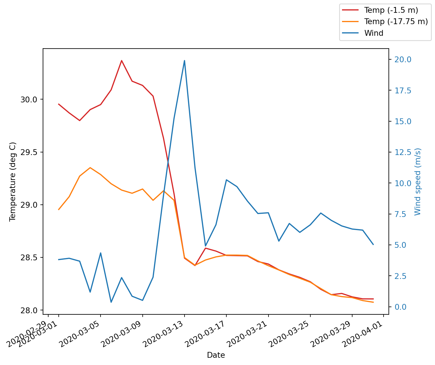

From this graph we can see that the surface water at Davies Reef was very warm during March 2020. There was a strong stratification of the temperature profile with cool water at -18 m. Around the 10th March the wind picked up for a few days, mixing the water, cooling the surface down rapidly.