import pandas as pd  # for data analysis
import numpy as np  # for quik maths
from janitor import clean_names  # to create consitent, 'clean' variable names
import folium  # a python API to interactive leaflet maps
import datetime as dt # to time how long the data export takes
from IPython.display import display # to render, i.e. 'display', html tables
from netCDF4 import DatasetAccess eReefs data
Programmatic server access
Learn how to extract eReefs data from the AIMS eReefs THREDDS server for multiple dates and points with OPeNDAP in Python .
This tutorial builds on the techniques introduced in Access eReefs data: Basic server access .
In this tutorial we will look at how to get eReefs data from the AIMS eReefs THREDDS server corresponding to the logged locations of tagged marine animals. Keep in mind, however, that the same methodology can be applied in any situation where we wish to extract eReefs data for a range of points with different dates of interest for each point.
Preparation
Create a folder named data.
Download the satellite tracking data file into your data folder.
Python modules
Motivating problem
The tracking of marine animals is commonly used by researchers to gain insights into the distribution, biology, behaviour and ecology of different species. However, knowing where an animal was at a certain point in time is only one piece of the puzzle. To start to understand why an animal was where it was, we usually require information on things like: What type of habitat is present at the location? What were the environmental conditions like at the time? What other lifeforms were present at the tracked location (e.g. for food or mating)?
In this tutorial we will pretend that we have tracking data for Loggerhead Sea Turtles and wish to get eReefs data corresponding to the tracked points (in time and space) to understand more about the likely environmental conditions experienced by our turtles.
Example tracking data
We will use satellite tracking data for Loggerhead Sea Turtles (Caretta caretta) provided in Strydom (2022). This data contains tracking detections which span the length of the Great Barrier Reef off the east coast of Queensland Australia from December 2021 to April 2022 (shown in Figure 1).
This dataset is a summarised representation of the tracking locations per 1-degree cell. This implies a coordinate uncertainty of roughly 110 km. This level of uncertainty renders the data virtually useless for most practical applications, though it will suffice for the purposes of this tutorial. Records which are landbased as a result of the uncertainty have been removed and from here on in we will just pretend that the coordinates are accurate.
# Read in data
data = pd.read_csv("data/Strydom_2022_DOI10-15468-k4s6ap.csv")

# Convert columns names from camelCase to snake_case
data = data.clean_names(case_type = "snake")

# Rename some variables for easier use
data = data.rename(columns = {
  "gbif_id": "record_id",
  "decimal_latitude": "latitude",
  "decimal_longitude": "longitude",
  "event_date": "date_time"
})

# Ensure date_time is in the datetime data format
data['date_time'] = pd.to_datetime(data['date_time'])

# Seperate date_time into date and time variables
data = data.assign(
  date = data['date_time'].dt.strftime("%Y-%m-%d"),
  time = data['date_time'].dt.strftime("%H:%M")
)

# Remove land based records (as a result of coordinate uncertainty)
land_based_records = [4022992331, 4022992326, 4022992312, 4022992315, 4022992322, 4022992306]
data = data.query("record_id not in @land_based_records")

# Select the variables relevant to this tutorial
select_vars = ["longitude", "latitude", "date", "time", "date_time","record_id", "species"]
data = data[select_vars]

# View the tracking locations on an interactive map:
# Create map centred on the mean coordinates of the tracking locations
centre_point = [data['latitude'].mean(), data['longitude'].mean()]
track_map = folium.Map(location = centre_point, zoom_start = 4)

# Add markers to map at each tracking location
for row in data.itertuples():
  coords_i = [row.latitude, row.longitude]
  marker_i = folium.Marker(
    location = coords_i,
    popup = row.date_time
  ).add_to(track_map)
To output the map from your Python script, you can add this line:
track_map.save('track_map.html')Make this Notebook Trusted to load map: File -> Trust Notebook
Extract data from server
We will extend the basic methods introduced in the preceding tutorial Accessing eReefs data from the AIMS eReefs THREDDS server to extract data for a set of points and dates.
We will extract the eReefs 1km hydrodynamic model daily mean temperature (temp), salinity (salt), and east- and northward current velocities (u and v) corresponding to the coordinates and dates for the tracking detections shown in Table 1.
# Create table of tracking detections (sort by date-time; select relevant variables)
tbl_detections = data.\
  sort_values('date_time')\
  [['date', 'time', 'longitude', 'latitude']]

# Output table in html format (hide row indices; format coordinates to their precision of 1 decimal place)
tbl_detections = tbl_detections.style.\
  hide(axis = 'index').\
  format(precision=1)
display(tbl_detections)
To output the detection table from your Python script, you can add this code:
with open('detections_table.html', 'w') as f:
f.write(tbl_detections.to_html())| date | time | longitude | latitude |
|---|---|---|---|
| 2021-12-21 | 17:57 | 152.5 | -24.5 |
| 2022-01-02 | 21:49 | 153.5 | -25.5 |
| 2022-01-05 | 07:33 | 152.5 | -23.5 |
| 2022-01-06 | 05:03 | 151.5 | -23.5 |
| 2022-01-09 | 20:25 | 151.5 | -22.5 |
| 2022-01-13 | 06:28 | 151.5 | -21.5 |
| 2022-01-14 | 18:26 | 150.5 | -21.5 |
| 2022-01-17 | 17:06 | 150.5 | -20.5 |
| 2022-01-19 | 17:44 | 149.5 | -20.5 |
| 2022-01-21 | 07:22 | 149.5 | -19.5 |
| 2022-01-23 | 07:02 | 148.5 | -19.5 |
| 2022-01-27 | 17:00 | 147.5 | -18.5 |
| 2022-01-30 | 17:02 | 146.5 | -18.5 |
| 2022-02-02 | 09:14 | 146.5 | -17.5 |
| 2022-02-03 | 21:37 | 153.5 | -24.5 |
| 2022-02-06 | 18:25 | 146.5 | -16.5 |
| 2022-02-07 | 07:15 | 145.5 | -16.5 |
| 2022-02-09 | 18:33 | 145.5 | -15.5 |
| 2022-02-12 | 08:59 | 153.5 | -26.5 |
| 2022-02-12 | 10:34 | 145.5 | -14.5 |
| 2022-03-25 | 07:10 | 144.5 | -13.5 |
| 2022-04-01 | 18:41 | 143.5 | -12.5 |
| 2022-04-09 | 22:00 | 143.5 | -11.5 |
| 2022-04-14 | 06:31 | 143.5 | -10.5 |
| 2022-04-21 | 10:30 | 143.5 | -9.5 |
We will take advantage of the consistent file naming on the server to extract the data of interest programmatically. We will first need to copy the OPeNDAP data link for one of the files within the correct model and aggregation folders and then replace the date.
Selecting a random date within the daily aggregated data (daily-daily; one data file per day) for the 1km hydro model (gbr1_2.0), we see the files have the naming format:
https://thredds.ereefs.aims.gov.au/thredds/dodsC/ereefs/gbr1_2.0/daily-daily/EREEFS_AIMS-CSIRO_gbr1_2.0_hydro_daily-daily-YYYY-MM-DD.nc
We will now write a script which extracts the data for the dates and coordinates in Table 1. For each unique date we will open the corresponding file on the server and extract the daily mean temperature, salinity, northward and southward current velocities for each set of coordinates corresponding to the date.
# GET DATA FOR EACH DATE AND COORDINATE (LAT LON) PAIR
t_start = dt.datetime.now() # to track run time of extraction

## 1. Setup variables for data extraction
# Server file name = <file_prefix><date (yyyy-mm-dd)><file_suffix>
file_prefix = "https://thredds.ereefs.aims.gov.au/thredds/dodsC/ereefs/gbr1_2.0/daily-daily/EREEFS_AIMS-CSIRO_gbr1_2.0_hydro_daily-daily-"
file_suffix = ".nc"

# Table of dates and coordinates for which to extract data (dates as character string)
detections = data[['date', 'longitude', 'latitude']].drop_duplicates()

extracted_data = pd.DataFrame() # to save the extracted data
dates = detections['date'].unique() # unique dates for which to open server files

## 2. For each date of interest, open a connection to the corresponding data file on the server
for i in range(len(dates)):
  date_i = dates[i]

  # Open file
  file_name_i = file_prefix + dates[i] + file_suffix
  server_file_i = Dataset(file_name_i)

  # Coordinates for which to extract data for the current date
  coordinates_i = detections.query("date == @date_i")

  # Get all coordinates in the open file (each representing the center-point of the corresponding grid cell)
  server_lons_i = server_file_i.variables['longitude'][:]
  server_lats_i = server_file_i.variables['latitude'][:]

  ## 3. For each coordinate (lon, lat) for the current date, get the data for the closest grid cell (1km^2) from the open server file
  for row_j in coordinates_i.itertuples():

    # Current coordinate of interest
    lon_j = row_j.longitude
    lat_j = row_j.latitude

    # Find the index of the grid cell containing our coordinate of interest (i.e. the center-point closest to our point of interest)
    lon_index_j = np.argmin(np.abs(server_lons_i - lon_j))
    lat_index_j = np.argmin(np.abs(server_lats_i - lat_j))
    # Note: This will return the closest grid cell, even for coordinates outside of the eReefs model boundary

    # Setup the dimension indices for which to extract data (needs to be a tuple; recall that python starts counting at 0)
    dim_ind = tuple([0, 15, lat_index_j, lon_index_j])
    ########################################
    # Recall the order of the dimensions (time, k, latitude, longitude) from the previous tutorial. Therefore we want [time = 1 (as we're using the daily files this is the only option), k = 15 corresponding to a depth of 0.5m, lat_index_j, lon_index_j]. If you are still confused, go back to the previous tutorial or have a look at the structure of one of the server files by uncommenting the following 5 lines of code:
    # not_yet_run = True  # used so the following lines are only run once
    # if not_yet_run:
    #   print(server_file_i.dimensions)
    #   print(server_file_i.variables)
    #   not_yet_run = False
    ########################################

    # Get the data for the grid cell containing our point of interest
    temp_j = server_file_i.variables['temp'][dim_ind]
    salt_j = server_file_i.variables['salt'][dim_ind]
    u_j = server_file_i.variables['u'][dim_ind]
    v_j = server_file_i.variables['v'][dim_ind]

    extracted_data_j = pd.DataFrame({
      'date': [date_i],
      'lon': [lon_j],
      'lat': [lat_j],
      'temp': [temp_j],
      'salt': [salt_j],
      'u': [u_j],
      'v': [v_j]
    })

    ## 4. Save data in memory and repeat for next date-coordinate pair
    extracted_data = pd.concat([extracted_data, extracted_data_j], ignore_index = True)

  # Close connection to open server file and move to the next date
  server_file_i.close()

# Calculate the run time of the extraction
t_stop = dt.datetime.now()
extract_time = t_stop - t_start
extract_mins = int(extract_time.total_seconds()/60)
extract_secs = int(extract_time.total_seconds() % 60)
print("Data extracted for", len(detections), "points from", len(dates), "files. \nExtraction time:", extract_mins, "min", extract_secs, "sec.")
Data extracted for 25 points from 24 files.
Extraction time: 1 min 5 sec.Our extracted data is shown below in Table 2.
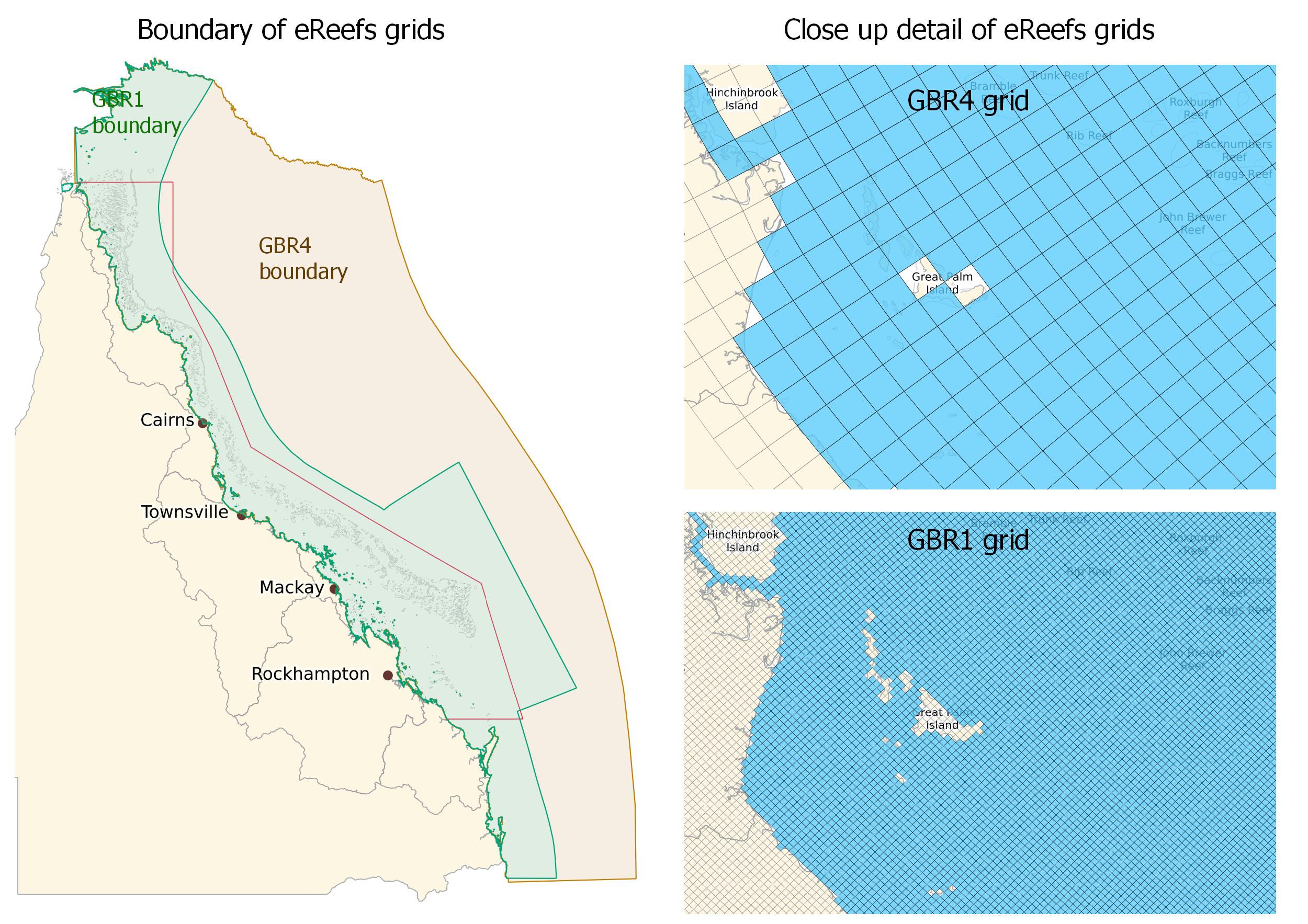
In the code above we match the closest eReefs model grid cell to each point in our list of coordinates (i.e. for each tracking detection). This will therefore match grid cells to all the coordinates, even if they are not within the eReefs model boundary. This behaviour may be useful when we have points right along the coastline as the eReefs models have small gaps at many points along the coast (see image below). However, in other cases this behaviour may not be desirable. For example, if we had points down near Sydney they would be matched to the closest eReefs grid cells (somewhere up near Brisbane) and the extracted data would be erroneous.
# Output table in html format (sort by date; hide row indices; format coordinates to their precision of 1 decimal place, temp & salt to 2 dp, u & v to 3 dp)
tbl_extracted = extracted_data.sort_values('date').style.\
  hide(axis = 'index').\
  format({
    **dict.fromkeys(['lon', 'lat'], '{:.1f}'),
    **dict.fromkeys(['temp', 'salt'], '{:.2f}'),
    **dict.fromkeys(['u', 'v'], '{:.3f}')
  })
display(tbl_extracted)
To output the extracted data table from your Python script, you can add this code:
with open('extracted_data_table.html', 'w') as f:
f.write(tbl_extracted.to_html())| date | lon | lat | temp | salt | u | v |
|---|---|---|---|---|---|---|
| 2021-12-21 | 152.5 | -24.5 | 28.09 | 35.26 | 0.071 | -0.020 |
| 2022-01-02 | 153.5 | -25.5 | 26.00 | 35.30 | -0.035 | 0.038 |
| 2022-01-05 | 152.5 | -23.5 | 25.64 | 35.23 | 0.030 | 0.015 |
| 2022-01-06 | 151.5 | -23.5 | 28.13 | 35.41 | -0.033 | 0.015 |
| 2022-01-09 | 151.5 | -22.5 | 29.24 | 35.34 | 0.001 | -0.103 |
| 2022-01-13 | 151.5 | -21.5 | 28.42 | 35.25 | -0.095 | 0.016 |
| 2022-01-14 | 150.5 | -21.5 | 28.99 | 35.40 | -0.064 | -0.047 |
| 2022-01-17 | 150.5 | -20.5 | 29.39 | 35.34 | -0.066 | -0.178 |
| 2022-01-19 | 149.5 | -20.5 | 29.92 | 35.48 | 0.018 | -0.104 |
| 2022-01-21 | 149.5 | -19.5 | 29.58 | 35.12 | -0.161 | -0.035 |
| 2022-01-23 | 148.5 | -19.5 | 28.99 | 35.26 | -0.137 | -0.022 |
| 2022-01-27 | 147.5 | -18.5 | 29.46 | 33.98 | 0.265 | 0.004 |
| 2022-01-30 | 146.5 | -18.5 | 30.15 | 34.60 | -0.184 | 0.143 |
| 2022-02-02 | 146.5 | -17.5 | 30.59 | 34.72 | 0.128 | -0.054 |
| 2022-02-03 | 153.5 | -24.5 | 27.06 | 35.32 | 0.550 | -0.797 |
| 2022-02-06 | 146.5 | -16.5 | 29.14 | 34.70 | -0.122 | -0.100 |
| 2022-02-07 | 145.5 | -16.5 | 30.37 | 34.06 | -0.104 | 0.200 |
| 2022-02-09 | 145.5 | -15.5 | 29.54 | 34.74 | -0.120 | 0.064 |
| 2022-02-12 | 153.5 | -26.5 | 26.80 | 35.38 | -0.124 | 0.006 |
| 2022-02-12 | 145.5 | -14.5 | 29.90 | 34.72 | -0.081 | 0.034 |
| 2022-03-25 | 144.5 | -13.5 | 29.04 | 34.75 | -0.457 | 0.360 |
| 2022-04-01 | 143.5 | -12.5 | 30.14 | 34.44 | 0.025 | -0.018 |
| 2022-04-09 | 143.5 | -11.5 | 29.93 | 34.56 | -0.097 | 0.144 |
| 2022-04-14 | 143.5 | -10.5 | 29.48 | 34.42 | -0.041 | 0.078 |
| 2022-04-21 | 143.5 | -9.5 | 29.56 | 34.19 | 0.059 | 0.034 |
Match extracted data to tracking data
We will match up the eReefs data with our tracking detections by combining the two datasets based on common date, longitude and latitude values.
# Rename lon and lat columns of extracted_data to longitude, latitude (to match those of data)
extracted_data = extracted_data.rename(columns = {
  'lon': 'longitude',
  'lat': 'latitude'
})

# Merge the two datasets based on common date, lon and lat values
combined_data = pd.merge(
  data, extracted_data,
  on = ['date', 'longitude', 'latitude']
)

# Print the combined data (reorder columns; sort by date and time; format numeric columns' decimal places)
tbl_combined = combined_data.\
  reindex(columns = ['date', 'time', 'longitude', 'latitude', 'record_id', 'temp', 'salt', 'u', 'v']).\
  sort_values(by = ['date', 'time']).\
  style.\
  hide(axis = 'index').\
  format({
    **dict.fromkeys(['longitude', 'latitude'], '{:.1f}'),
    **dict.fromkeys(['temp', 'salt'], '{:.2f}'),
    **dict.fromkeys(['u', 'v'], '{:.3f}')
  })
display(tbl_combined)
To output the combined data table from your Python script, you can add this code:
with open('combined_data_table.html', 'w') as f:
f.write(tbl_combined.to_html())| date | time | longitude | latitude | record_id | temp | salt | u | v |
|---|---|---|---|---|---|---|---|---|
| 2021-12-21 | 17:57 | 152.5 | -24.5 | 4022992328 | 28.09 | 35.26 | 0.071 | -0.020 |
| 2022-01-02 | 21:49 | 153.5 | -25.5 | 4022992329 | 26.00 | 35.30 | -0.035 | 0.038 |
| 2022-01-05 | 07:33 | 152.5 | -23.5 | 4022992304 | 25.64 | 35.23 | 0.030 | 0.015 |
| 2022-01-06 | 05:03 | 151.5 | -23.5 | 4022992302 | 28.13 | 35.41 | -0.033 | 0.015 |
| 2022-01-09 | 20:25 | 151.5 | -22.5 | 4022992319 | 29.24 | 35.34 | 0.001 | -0.103 |
| 2022-01-13 | 06:28 | 151.5 | -21.5 | 4022992308 | 28.42 | 35.25 | -0.095 | 0.016 |
| 2022-01-14 | 18:26 | 150.5 | -21.5 | 4022992318 | 28.99 | 35.40 | -0.064 | -0.047 |
| 2022-01-17 | 17:06 | 150.5 | -20.5 | 4022992330 | 29.39 | 35.34 | -0.066 | -0.178 |
| 2022-01-19 | 17:44 | 149.5 | -20.5 | 4022992320 | 29.92 | 35.48 | 0.018 | -0.104 |
| 2022-01-21 | 07:22 | 149.5 | -19.5 | 4022992316 | 29.58 | 35.12 | -0.161 | -0.035 |
| 2022-01-23 | 07:02 | 148.5 | -19.5 | 4022992323 | 28.99 | 35.26 | -0.137 | -0.022 |
| 2022-01-27 | 17:00 | 147.5 | -18.5 | 4022992327 | 29.46 | 33.98 | 0.265 | 0.004 |
| 2022-01-30 | 17:02 | 146.5 | -18.5 | 4022992314 | 30.15 | 34.60 | -0.184 | 0.143 |
| 2022-02-02 | 09:14 | 146.5 | -17.5 | 4022992301 | 30.59 | 34.72 | 0.128 | -0.054 |
| 2022-02-03 | 21:37 | 153.5 | -24.5 | 4022992313 | 27.06 | 35.32 | 0.550 | -0.797 |
| 2022-02-06 | 18:25 | 146.5 | -16.5 | 4022992303 | 29.14 | 34.70 | -0.122 | -0.100 |
| 2022-02-07 | 07:15 | 145.5 | -16.5 | 4022992310 | 30.37 | 34.06 | -0.104 | 0.200 |
| 2022-02-09 | 18:33 | 145.5 | -15.5 | 4022992311 | 29.54 | 34.74 | -0.120 | 0.064 |
| 2022-02-12 | 08:59 | 153.5 | -26.5 | 4022992324 | 26.80 | 35.38 | -0.124 | 0.006 |
| 2022-02-12 | 10:34 | 145.5 | -14.5 | 4022992325 | 29.90 | 34.72 | -0.081 | 0.034 |
| 2022-03-25 | 07:10 | 144.5 | -13.5 | 4022992309 | 29.04 | 34.75 | -0.457 | 0.360 |
| 2022-04-01 | 18:41 | 143.5 | -12.5 | 4022992307 | 30.14 | 34.44 | 0.025 | -0.018 |
| 2022-04-09 | 22:00 | 143.5 | -11.5 | 4022992317 | 29.93 | 34.56 | -0.097 | 0.144 |
| 2022-04-14 | 06:31 | 143.5 | -10.5 | 4022992321 | 29.48 | 34.42 | -0.041 | 0.078 |
| 2022-04-21 | 10:30 | 143.5 | -9.5 | 4022992305 | 29.56 | 34.19 | 0.059 | 0.034 |
Hooray! We now have our combined dataset of the Loggerhead Sea Turtle tracking detections and the corresponding eReefs daily aggregated data (Table 3).
Strydom A. 2022. Wreck Rock Turtle Care - satellite tracking. Data downloaded from OBIS-SEAMAP; originated from Satellite Tracking and Analysis Tool (STAT). DOI: 10.15468/k4s6ap accessed via GBIF.org on 2023-02-17.