Analysis

Note

This page covers functions provided by ADRIAanalysis. Ensure it is installed before running the examples (see Getting Started).

Warning

Examples of analysis and visualizations are still being developed, so take the examples below as illustrations of what analysis and visualizations are possible, but not the intended quality. Caution is advised when interpreting results as they are misleading without in-depth assessment.

This section presents tools for analysing model generated data, including functions to extract metrics and plot graphs.

Setup

Plotly is recommended for quick visual assessment, however the Makie backend is more suitable for publication quality plots.

While we use Plotly for the code here, the equivalent figures from Makie are shown.

Install PlotlyBase alongside ADRIAviz and ADRIAanalysis:

julia> ]add ADRIAviz ADRIAanalysis PlotlyBase
julia> ]add PlotlyKaleido  # optional, enables static image export

Load and activate the Plotly backend before calling any visualization function:

using ADRIA, ADRIAviz, ADRIAanalysis, PlotlyBase
ADRIAviz.activate("plotly")

using Statistics

ResultSet

All metrics and visualization tools presented here can be used with data generated from ADRIA. The examples below assume an ADRIAResultSet rs:

dom = ADRIA.load_domain("path to domain data", "<RCP>")

num_samples = 4096
scens = ADRIA.sample(dom, num_samples)

rcp_45 = "45"
rs = ADRIA.run_scenarios(dom, scens, rcp_45)

s_tac = ADRIA.metrics.scenario_total_cover(rs)
ADRIA.viz.scenarios(rs, s_tac)

If using the Plotly backend, a separate call to display the figure is needed
fig = ADRIA.viz.scenarios(rs, s_tac)
ADRIA.viz.show_in_browser(fig)

See the previous sections Loading a Domain, Generating scenarios and Running scenarios for more information.

Extracting results

A range of metrics are defined as part of the ADRIA framework. See the Metrics page for more details.

The following extracts results for specific metrics for each timestep and site across all scenarios. Each result is a 3-dimensional Array of timesteps, sites and scenarios:

tac = ADRIA.metrics.total_absolute_cover(rs)
rsv = ADRIA.metrics.relative_shelter_volume(rs)
juves = ADRIA.metrics.relative_juveniles(rs)

Scenario-level metrics aggregate the above across the site dimension and indicate the outcomes under a given intervention (or non-intervention) option and environmental condition. The result is a 2-dimensional array of timesteps and scenarios:

s_tac = ADRIA.metrics.scenario_total_cover(rs)
s_rsv = ADRIA.metrics.scenario_rsv(rs)
s_juves = ADRIA.metrics.scenario_relative_juveniles(rs)

Visualization

The examples below illustrate usage. For further information on each method of analysis, see the documentation for the given function.

Some shared options used by the plots below:

fig_opts = Dict(:size => (1600, 800))

opts = Dict(
    :factors => [
        :RCP,
        :dhw_scenario,
        :wave_scenario,
        :guided,
        :mcda_method,
        :N_seed_TA,
        :N_seed_CA,
        :fogging,
        :SRM,
        :a_adapt
    ]
)

Scenario outcomes

Plot a quick scenario overview:

fig_s_tac = ADRIA.viz.scenarios(
    rs, s_tac; fig_opts=fig_opts, axis_opts=Dict(:ylabel => "Scenario Total Cover")
)
ADRIA.viz.savefig(fig_s_tac, "scenarios_tac.html")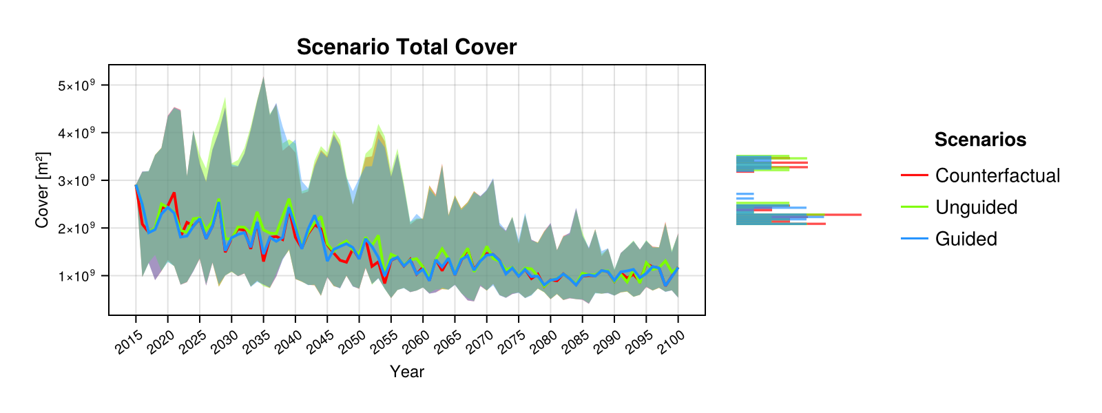

Intervention location selection - visualisation

Plot spatial colormaps of site selection frequencies and other available site selection metrics.

# Calculate frequencies with which each site was selected at each rank
rank_freq = ADRIA.decision.ranks_to_frequencies(ADRIA.metrics.seed_ranks(rs))

# Plot 1st rank frequencies as a colormap
rank_fig = ADRIA.viz.ranks_to_frequencies(rs, rank_freq, 1; fig_opts=Dict(:size=>(1200, 800)))
ADRIA.viz.savefig(rank_fig, "single_rank_plot.html")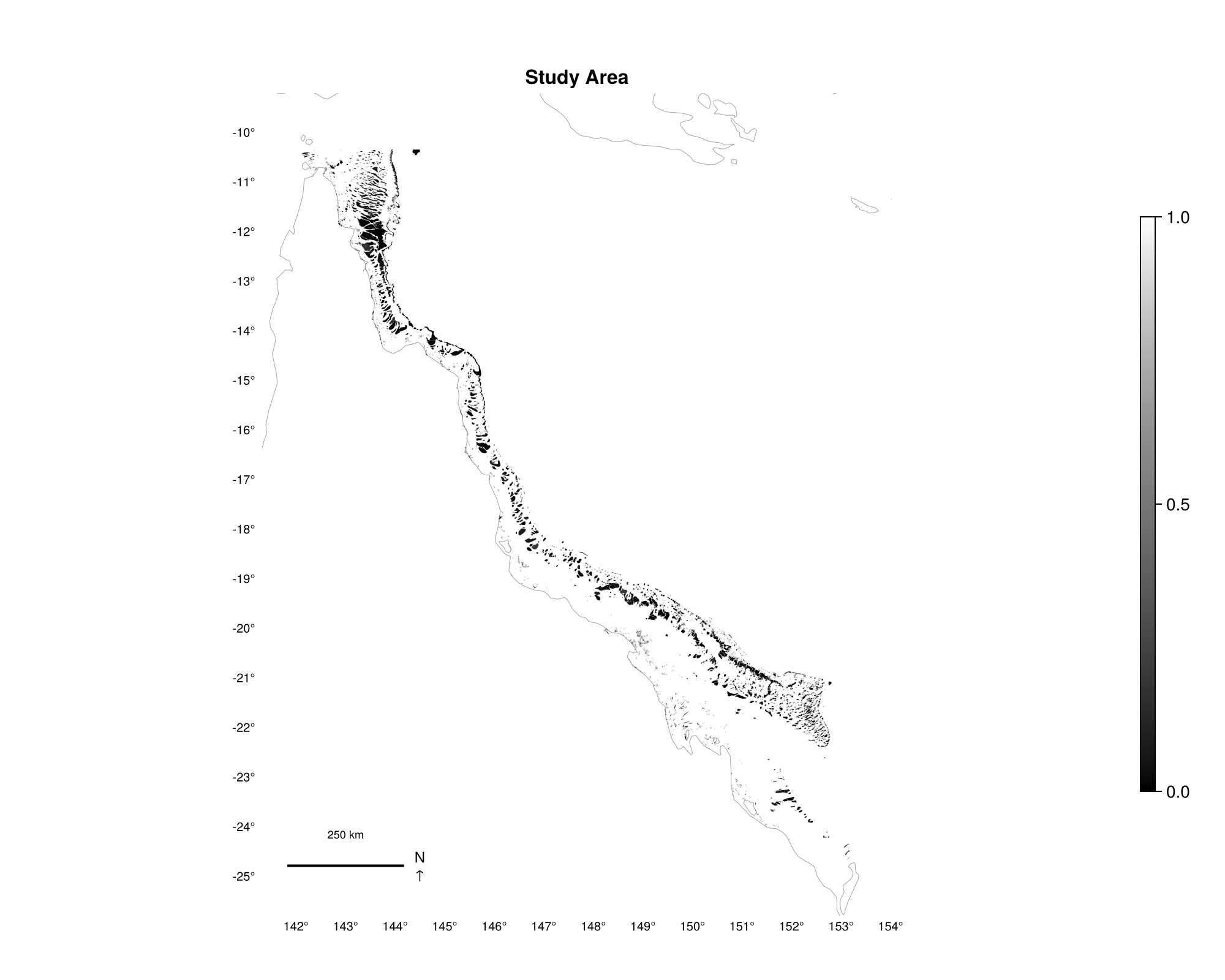

# Plot 1st, 2nd and 3rd rank frequencies as an overlayed colormap
rank_fig = ADRIA.viz.ranks_to_frequencies(rs, rank_freq, [1, 2, 3]; fig_opts=Dict(:size=>(1200, 800)))
ADRIA.viz.savefig(rank_fig, "ranks_plot.html")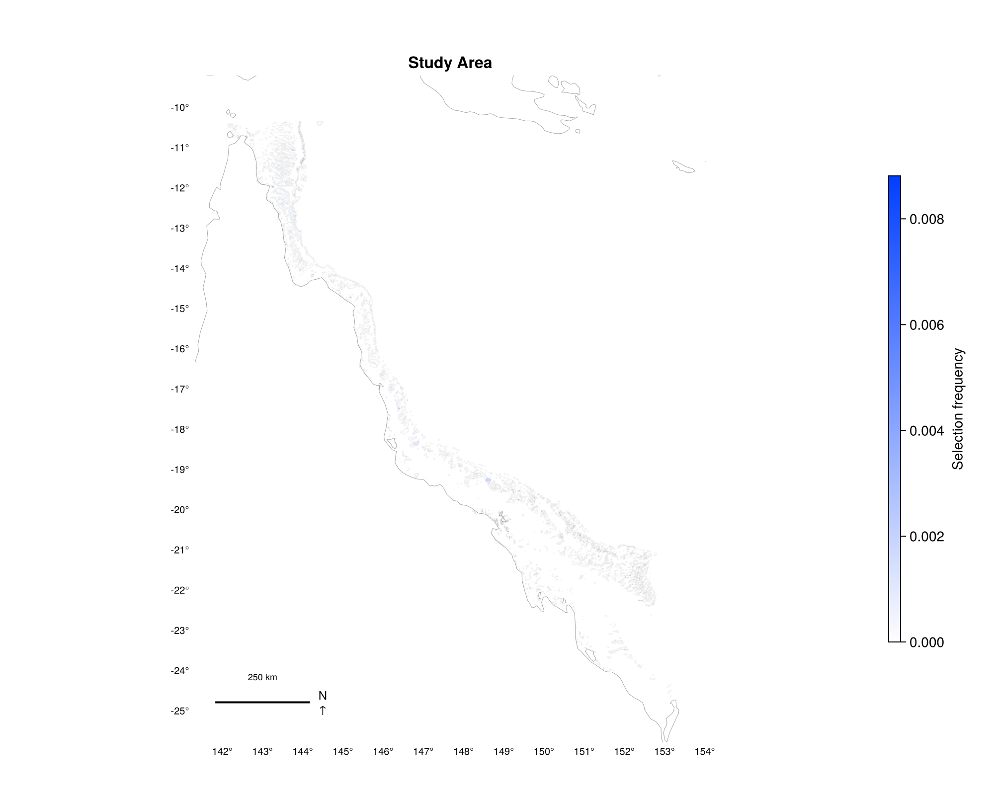

Intervention location selection - plot criteria maps

mcda_funcs = ADRIA.decision.mcda_methods()

dom = ADRIA.load_domain("path to domain", "45")

scens = ADRIA.sample_guided(dom, 2^2)
scen = scens[1, :]

# Get seeding preferences
seed_pref = ADRIA.decision.SeedPreferences(dom, scen)

# Calculate criteria vectors
sum_cover = vec(sum(dom.init_coral_cover; dims=1).data)
dhw_scens = dom.dhw_scens[:, :, Int64(scen["dhw_scenario"])]
plan_horizon = Int64(scen["plan_horizon"])
projection_confidence = scen["projection_confidence"]
decay = ADRIA.decision.build_decay(plan_horizon, projection_confidence)
dhw_projection = ADRIA.decision.weighted_projection(dhw_scens, 1, plan_horizon, decay, 75)
area_weighted_conn = dom.conn.data .* ADRIA.loc_k_area(dom)
conn_cache = similar(area_weighted_conn)
in_conn, out_conn, network = ADRIA.connectivity_strength(
    area_weighted_conn, sum_cover, conn_cache
)

# Create decision matrix
seed_decision_mat = ADRIA.decision.decision_matrix(
    dom.loc_ids,
    seed_pref.names;
    seed_in_connectivity=in_conn,
    seed_out_connectivity=out_conn,
    seed_heat_stress=dhw_projection,
    seed_coral_cover=sum_cover
)

# Get results from applying MCDA algorithm
crit_agg = ADRIA.decision.criteria_aggregated_scores(
    seed_pref, seed_decision_mat, mcda_funcs[1]
)

# Don't plot constant criteria
is_const = Bool[length(x) == 1 for x in unique.(eachcol(seed_decision_mat.data))]

# Plot normalized scores and criteria as map
fig = ADRIA.viz.selection_criteria_map(
    dom, seed_decision_mat[criteria=.!is_const], crit_agg.scores ./ maximum(crit_agg.scores)
)
ADRIA.viz.savefig(fig, "criteria_plots.html")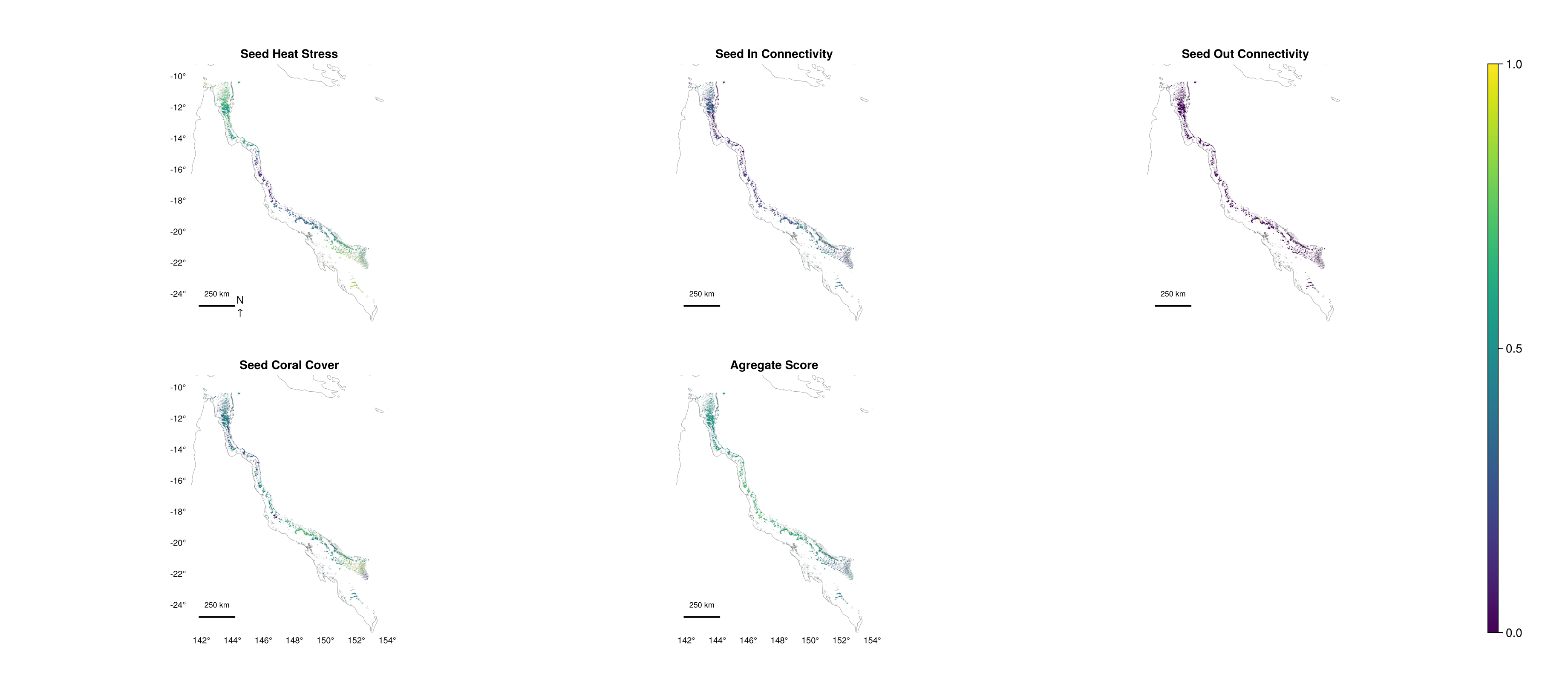

PAWN sensitivity (heatmap overview)

The PAWN sensitivity analysis method is a moment-independent approach to Global Sensitivity Analysis. It is described as producing robust results at relatively low sample sizes, and is used to screen factors (i.e., identification of important factors) and rank factors as well (ordering factors by their relative contribution towards a given quantity of interest).

# Sensitivity of mean scenario outcomes to factors
mean_s_tac = vec(mean(s_tac, dims=1))
tac_Si = pawn(rs, mean_s_tac)
pawn_fig = ADRIA.viz.pawn(tac_Si; opts, fig_opts)
ADRIA.viz.savefig(pawn_fig, "pawn_si.html")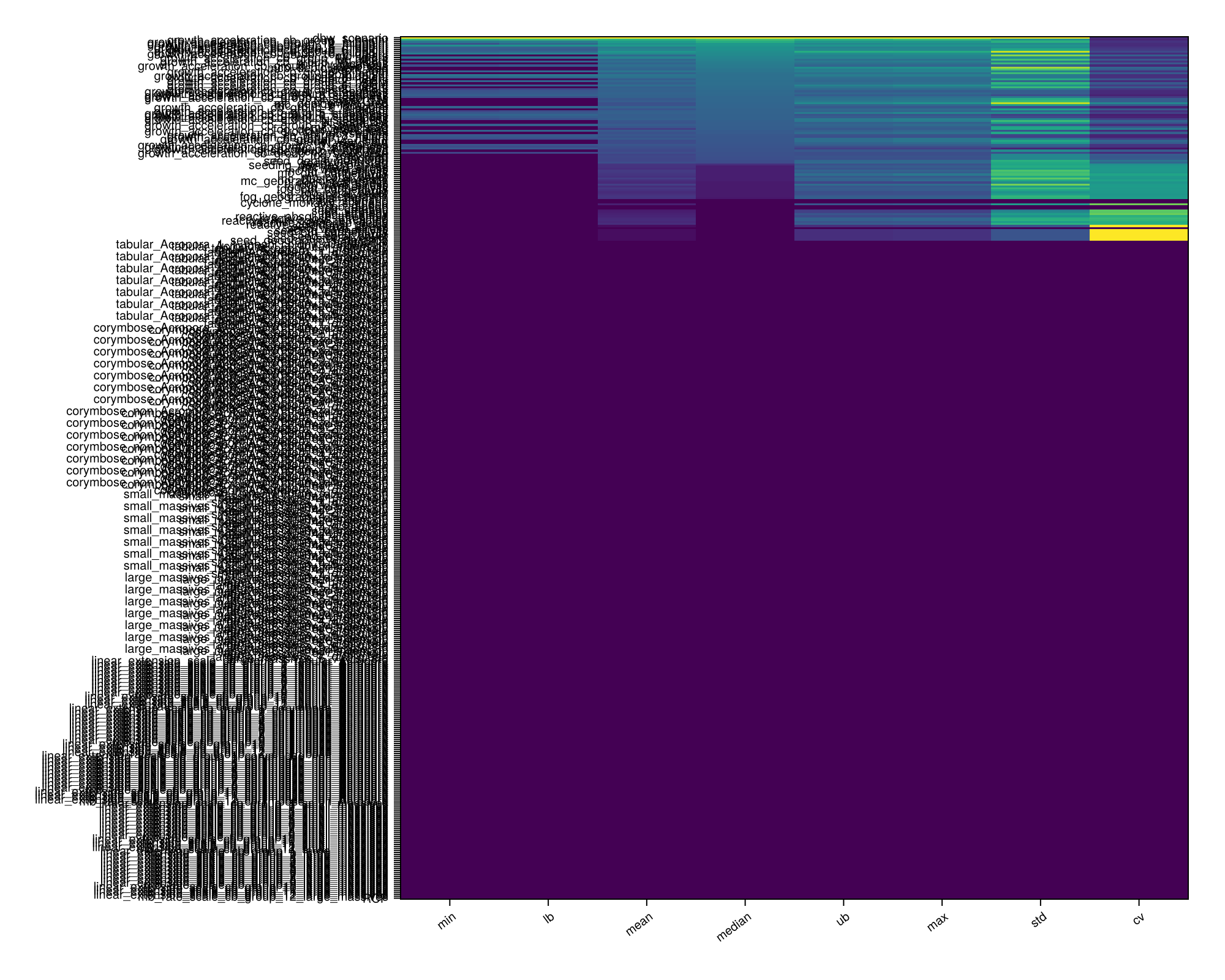

Temporal Sensitivity Analysis

Temporal (or Time-varying) Sensitivity Analysis applies sensitivity analysis to model outputs over time. The relative importance of factors and their influence on outputs over time can then be examined through this analysis.

tsa_s = tsa(rs, s_tac)
tsa_fig = ADRIA.viz.tsa(rs, tsa_s; opts, fig_opts)
ADRIA.viz.savefig(tsa_fig, "tsa.html")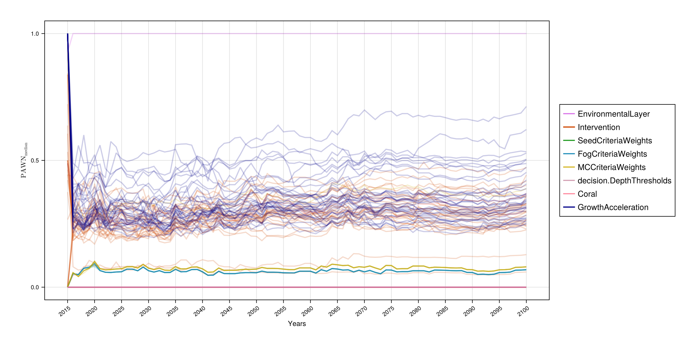

Convergence Analysis

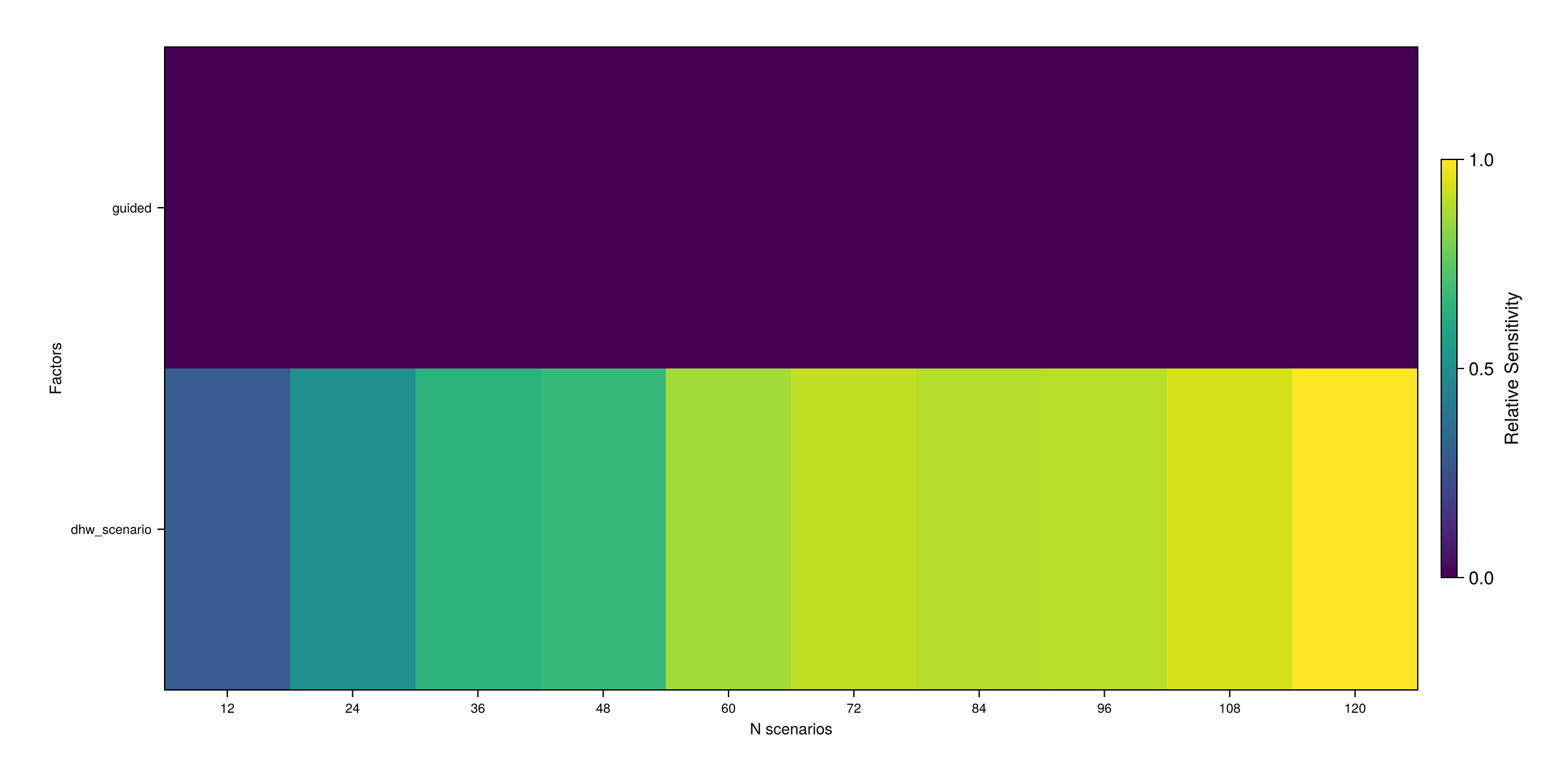
When undertaking sensitivity analysis it is important to have a sufficient number of samples such that the sensitivity measure converges to a stable state. To assess whether sufficient samples have been taken a convergence analysis can be conducted. One approach is to draw a large sample and then iteratively assess stability of the sensitivity metric using an increasing number of sub-samples. The sensitivity metric is described as having "converged" if there is little to no fluctuations/variance for a given sample size. The analysis can help determine if too little (or too many) samples have taken for the purpose of sensitivity analysis.

The function sensitivity.convergence can be used to calculate a sensitivity measure for an increasing number of samples. The result can then be plotted as band plots or a heat map using viz.convergence.

outcome = dropdims(mean(s_tac; dims=:timesteps); dims=:timesteps)

# Display convergence for specific factors of interest ("foi") within a single figure.
# Bands represent the 95% confidence interval derived from the number of conditioning
# points (default is 10 samples).
foi = [:dhw_scenario, :wave_scenario, :guided, :mcda_method]
Si_conv = convergence(scens, outcome, foi)
conv_series_fig = ADRIA.viz.convergence(Si_conv, foi)
ADRIA.viz.savefig(conv_series_fig, "convergence_factors_series.html")

# Convergence analysis of factors grouped by model component as a heat map
components = [:EnvironmentalLayer, :Intervention, :Coral]
Si_conv = convergence(scens, outcome, components)
conv_hm_fig = ADRIA.viz.convergence(Si_conv, components; opts=Dict(:viz_type=>:heatmap))
ADRIA.viz.savefig(conv_hm_fig, "convergence_components_heatmap.html")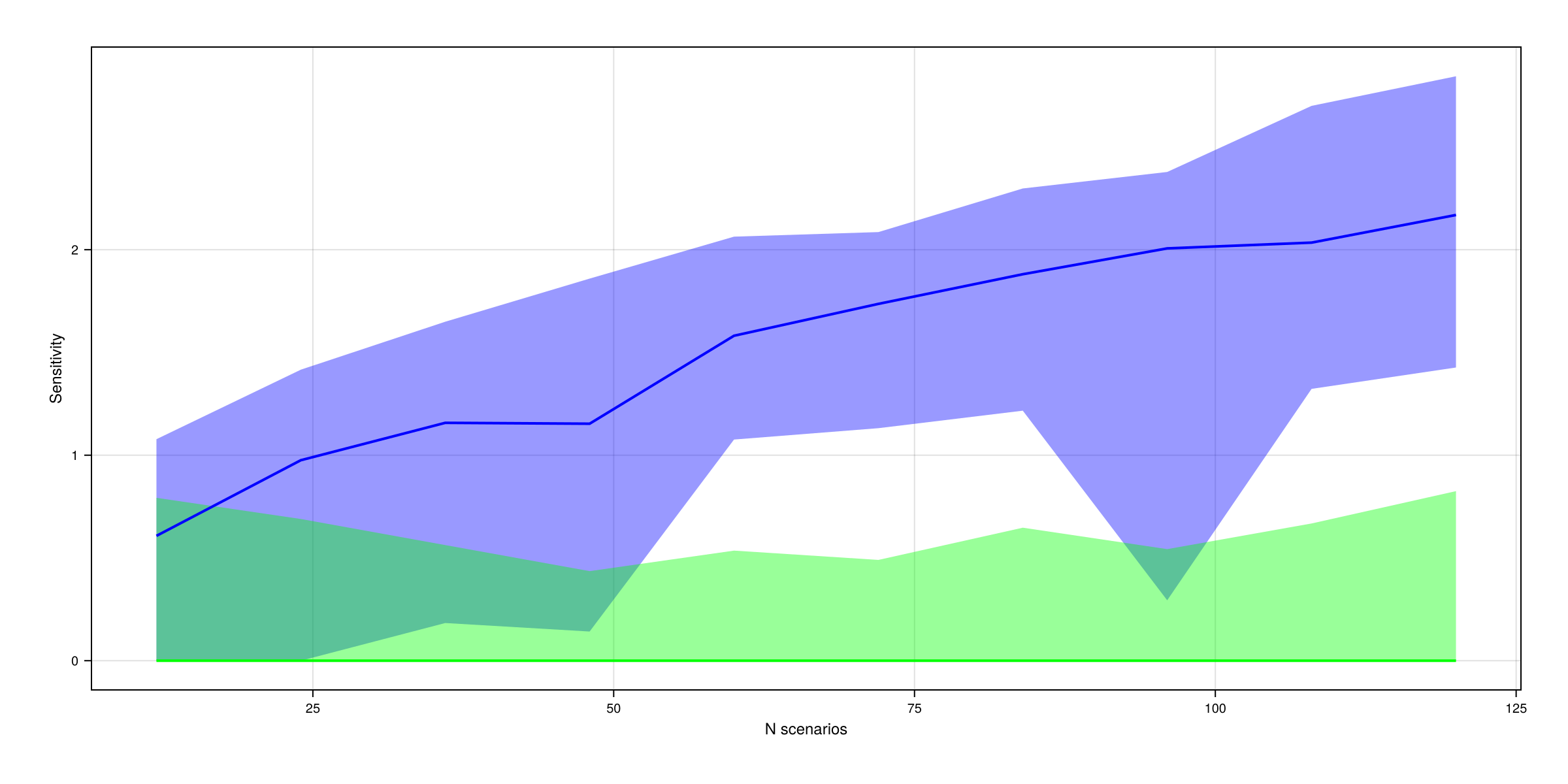

Time Series Clustering

The Time Series Clustering algorithm clusters together series (typically time series) with similar behavior. This is achieved by computing the Euclidian distance between each pair of series weighted by a correlation factor that takes into account the quotient between their complexities. When plotting clustered_scenarios, the kwarg opts can be used with the key :summarize to plot the confidence intervals of each cluster instead of each series individually (default is true).

s_tac = ADRIA.metrics.scenario_total_cover(rs)

n_clusters = 4
clusters = cluster_scenarios(s_tac, n_clusters)

axis_opts = Dict(
    :title => "Time Series Clustering with $n_clusters clusters",
    :ylabel => "TAC [m2]",
    :xlabel => "Timesteps [years]",
)
opts = Dict{Symbol, Any}(:summarize => true)

tsc_fig = ADRIA.viz.clustered_scenarios(
    s_tac, clusters; opts=opts, fig_opts=fig_opts, axis_opts=axis_opts
)
ADRIA.viz.savefig(tsc_fig, "tsc.html")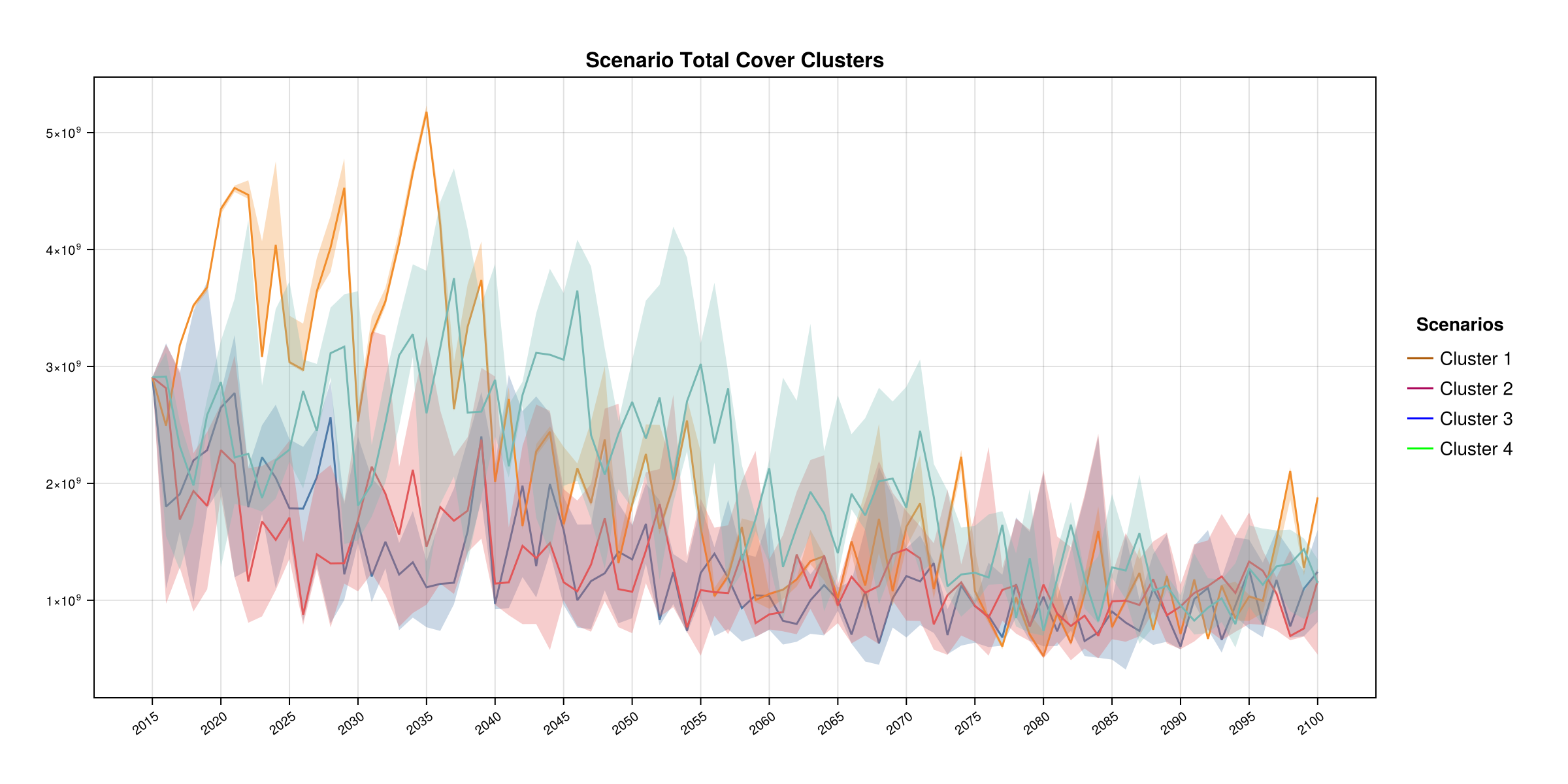

Target clusters

One can also target scenarios that belong to specific clusters (like clusters with higher median value for some outcome).

Here we use clustering to identify groups of time series for sites with low temporal variability in shelter volume across scenarios.

# Time series for each site summarizing median shelter volume across all scenarios
asv = ADRIA.metrics.absolute_shelter_volume(rs)
asv_site_series = ADRIA.metrics.loc_trajectory(median, asv)

# Cluster sites with similar shelter volume time series
n_clusters = 6
asv_clusters = cluster_series(asv_site_series, n_clusters)

# find_scenarios computes median timeseries for each cluster
#   and by default calculates temporal variability of that median timeseries
# Target sites that belong to the two clusters with lowest temporal variability
lowest = x -> x .∈ [sort(x; rev=true)[1:2]]
asv_target = find_scenarios(asv_site_series, asv_clusters, lowest)

axis_opts = Dict(:ylabel => "Absolute Shelter Volume", :xlabel => "Timesteps [years]")

tsc_asc_fig = ADRIA.viz.clustered_scenarios(
    asv_site_series, asv_target; axis_opts=axis_opts, fig_opts=fig_opts
)
ADRIA.viz.savefig(tsc_asc_fig, "tsc_asv.html")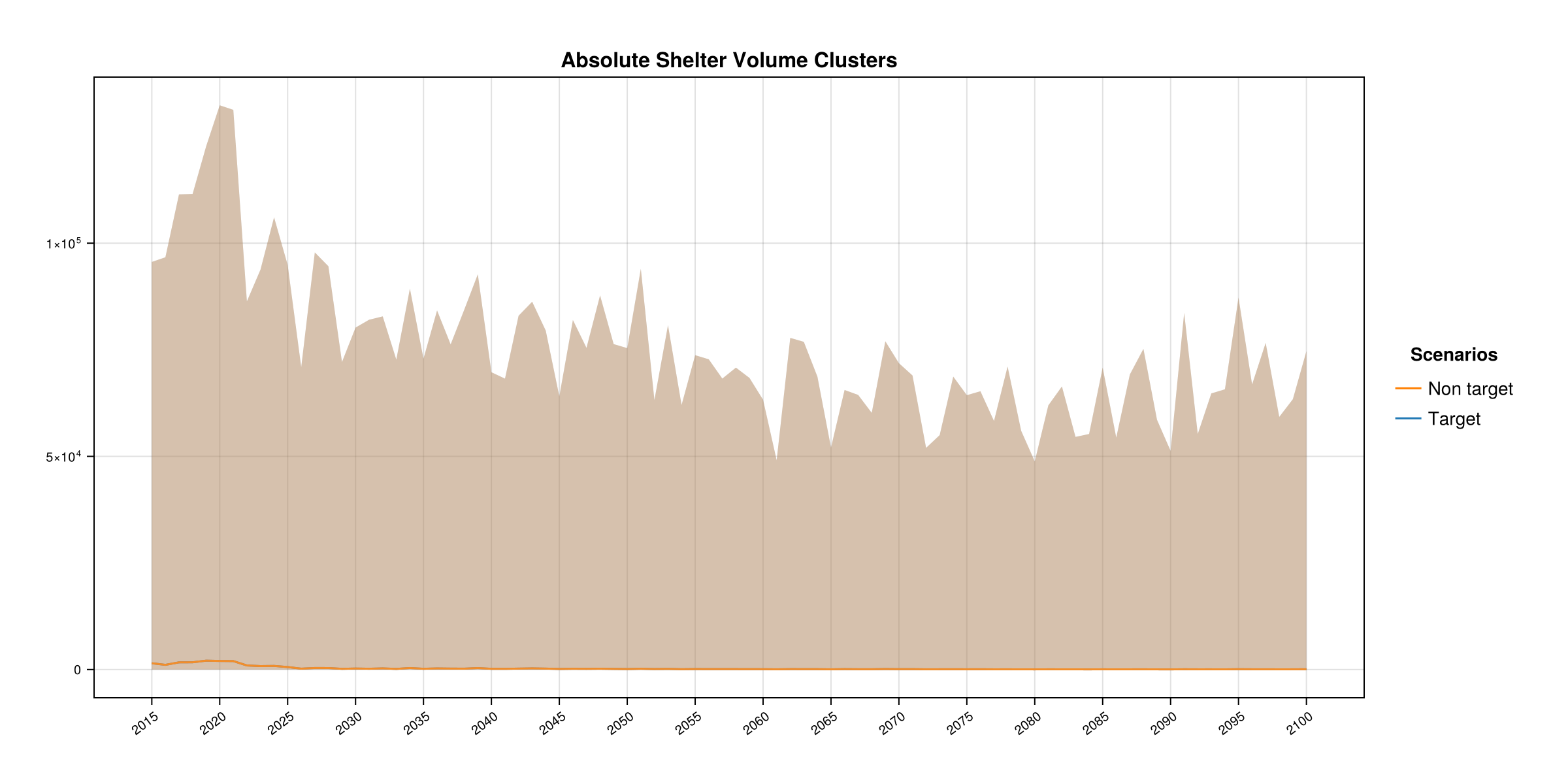

As expected, we see the sites in the target group have lower temporal variability. The non-target group has larger temporal variability. The sites could then be investigated further.

As the sites were selected using the median timeseries of two clusters, there is still a large range of shelter volume across sites at the start of the time series. Focusing on the lowest cluster or splitting into more clusters could produce a more homogeneous group of scenarios.

This can be interpreted as a form of scenario discovery where a target group of timeseries is summarised visually. Here the timeseries represent sites rather than scenarios. Using summarize, timeseries for scenarios could be obtained by aggregating over sites.

For this test dataset, findings in terms of scenario discovery suggest:

1. Ensuring conditions for success: Low temporal variability in shelter volume involves sites that stay low. Temporal variability would likely not be interpreted as a success metric given that high temporal variability also reflects large declines in shelter volume.

2. Avoiding failure: Both groups show declines across all sites using the median across scenarios. The analysis could be repeated to investigate how behaviour differs across scenarios, particularly in which interventions improve outcomes.

3. Planning for failure modes: The non-target group of sites starts with higher shelter volume. While the median across scenarios declines, further investigation could test whether certain interventions cope better than others with changing conditions.

4. Further deliberation: Discussion would likely further explore performance metrics other than temporal variability, and factors other than sites.

Multiple Time Series Clustering

It is possible to perform time series clustering for different metric outcomes and find scenarios that behave the same across all of them. Currently there is no visualization function for this.

metrics::Vector{ADRIA.metrics.Metric} = [
    ADRIA.metrics.scenario_total_cover,
    ADRIA.metrics.scenario_asv,
    ADRIA.metrics.scenario_absolute_juveniles,
]

outcomes = ADRIA.metrics.scenario_outcomes(rs, metrics)
n_clusters = 6

# Clusters matrix
outcomes_clusters::AbstractMatrix{Int64} = cluster_scenarios(outcomes, n_clusters)

# Filter scenarios that belong to one of the 4 high value clusters for all outcomes
highest_clusters(x) = x .∈ [sort(x; rev=true)[1:4]]
robust_scens = find_scenarios(outcomes, outcomes_clusters, highest_clusters)

Time Series Clustering Map

When using Time Series Clustering to cluster among multiple locations using some metric, it is possible to visualize the result as a map.

tac = ADRIA.metrics.total_absolute_cover(rs)

# Get a timeseries summarizing the scenarios for each site
tac_site_series = ADRIA.metrics.loc_trajectory(median, tac)

n_clusters = 6
clusters = ADRIA.analysis.cluster_scenarios(tac_site_series, n_clusters)

# Get a vector summarizing the scenarios and timesteps for each site
tac_sites = ADRIA.metrics.per_loc(median, tac)

tsc_map_fig = ADRIA.viz.map(rs, tac_sites, clusters)
ADRIA.viz.savefig(tsc_map_fig, "tsc_map.html")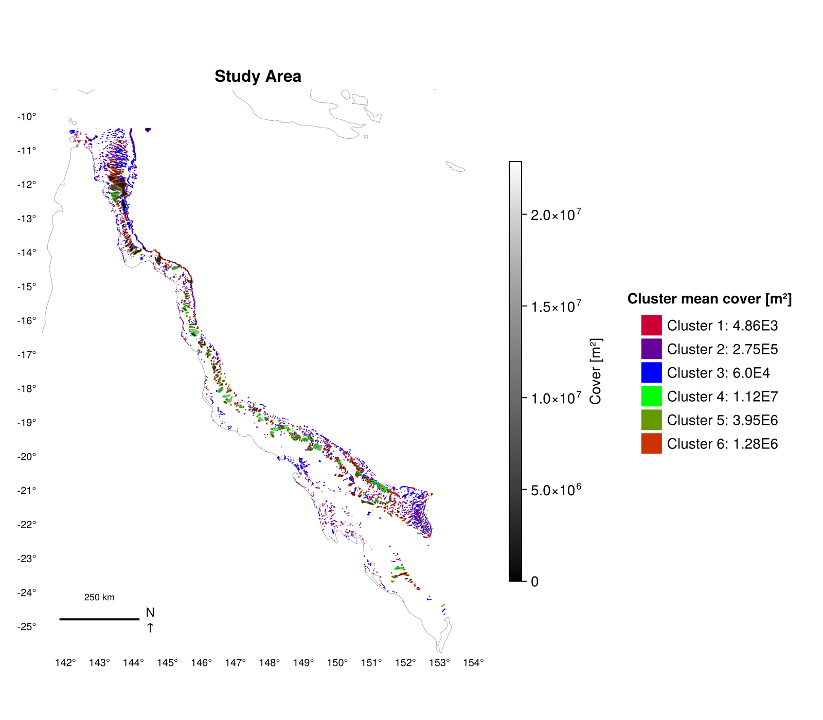

Rule Induction (using Series Clusters)

The SIRUS Rule Induction algorithm (Benard et al. 2021) can be used for scenario discovery by summarising scenarios in terms of binary rules, i.e. thresholds below/above which a factor will lead to a specified outcome.

For this example, we cluster scenarios with similar total cover, and then focus on those with high temporal variability in total cover. We explore what intervention characteristics lead to high temporal variability.

s_tac = ADRIA.metrics.scenario_total_cover(rs)
n_clusters = 6
clusters = cluster_scenarios(s_tac, n_clusters)

# Identify cluster(s) with highest median temporal variability covering at least 1% of scenarios
tgt = target_clusters(clusters, s_tac)

When the SIRUS Rule Induction algorithm produces rules involving two factors, they can be visualised as scatterplots.

rule_foi = ADRIA.component_params(rs, [Intervention, SeedCriteriaWeights]).fieldname

max_rules = 10
rules_iv = cluster_rules(
    rs, tgt, scens, rule_foi, max_rules; remove_duplicates=true
)

rules_scatter_fig = ADRIA.viz.rules_scatter(
    rs,
    scens,
    tgt,
    rules_iv;
    fig_opts=fig_opts,
    opts=opts
)
ADRIA.viz.savefig(rules_scatter_fig, "rules_scatter.html")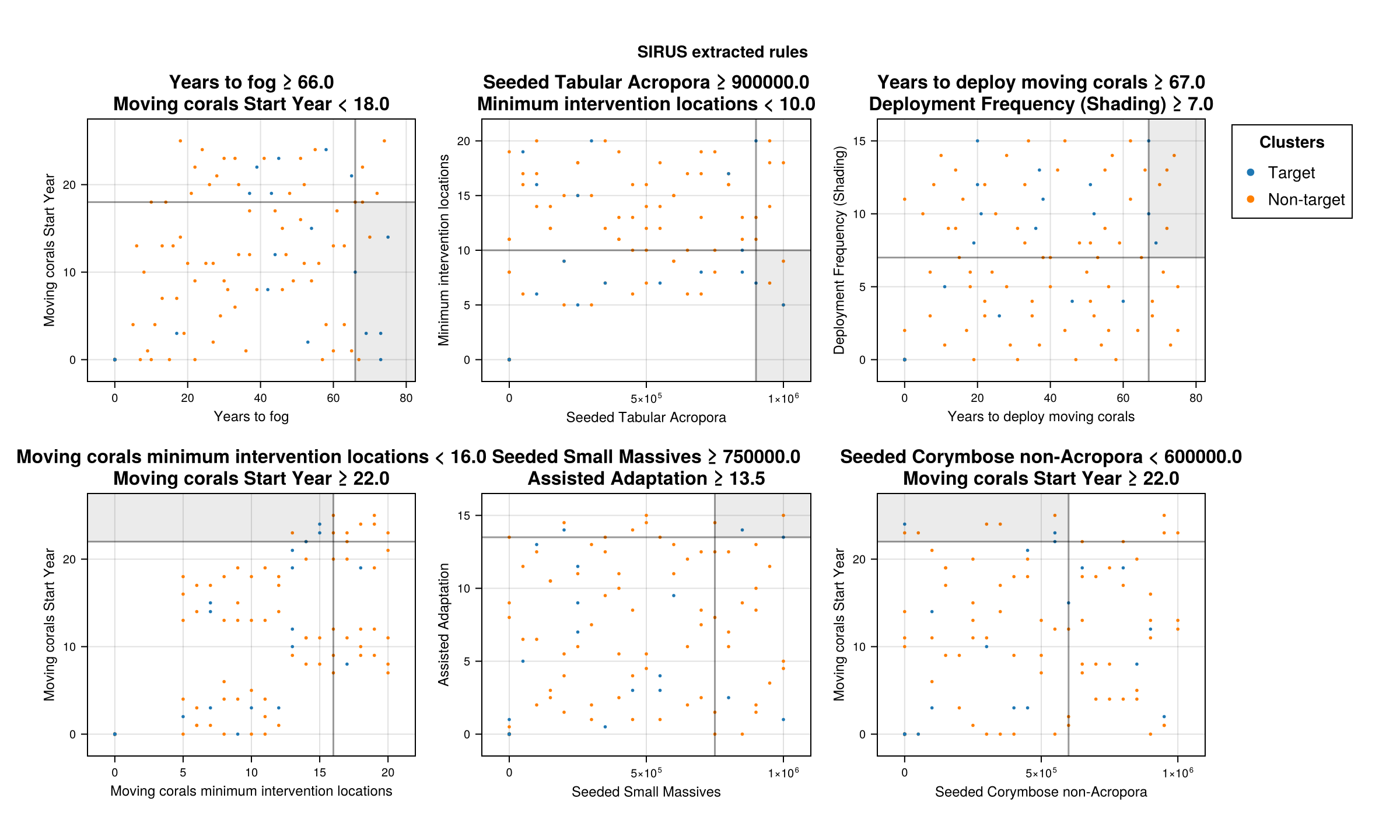

When defining binary rules, it is expected that there will be a tradeoff between coverage and density (Bryant & Lempert 2010). Not all target scenarios will be captured (low coverage), and not all scenarios captured by the rule will be target scenarios (low density). It is possible for a rule to increase coverage by accepting lower density, and density can often be increased by accepting lower coverage.

In these results, a number of rules have many blue points outside the grey area - the rule has low coverage of the target scenarios, e.g., in SRM > 3.94 & Years to Shade > 54.0.

A number of rules also have many orange points within the grey area - the rule has low density of target scenarios, e.g., SRM > 3.94 & Years to Shade > 38.0.

SRM and Years to Shade have been selected as key factors in several of the rules. In this dataset, high temporal variability is obtained when a large reduction in DHW is applied, and for a long period of time. This may reflect a large increase in coral cover - but would need further investigation.

Rules also suggest that high temporal variability is also obtained when putting high weight on selecting locations with high outgoing connectivity and low coral cover - in combination with high shading. The rule favouring low coral cover has very low coverage - there are many target scenarios that also do not have low coral cover.

For this dataset, according to this analysis:

1. Ensuring conditions for success: Temporal variability might be a proxy for high improvement over time, and the scenarios could be visualised or another more specific metric could be used to verify this. It would be unsurprising for high shading to support success.

2. Avoiding failure: Binary rules implicitly define scenarios that are excluded. High temporal variability is rarely achieved without high levels of shade.

3. Planning for failure modes: A recommendation to favour locations with high outgoing connectivity combined with high SRM seems like it would warrant further investigation - the rule includes many target scenarios (high coverage), but also many scenarios with lower temporal variability (high density).

4. Further deliberation: The rules describe very high levels of shading for long periods of time, which may be difficult to achieve. Temporal variability is not directly connected with measures of success - alternative metrics to summarise clusters could be explored. Other algorithms, e.g., PRIM, could also be used to give greater control over coverage and density (Bryant & Lempert 2010).

Regional Sensitivity Analysis

Regional Sensitivity Analysis visualises how two factors jointly relate to an outcome. Scenarios are plotted as a 2D scatter of two factors of interest, coloured by outcome value.

using ADRIAanalysis

s_tac = ADRIA.metrics.scenario_total_cover(rs)
mean_s_tac = vec(mean(s_tac; dims=1))

# Build feature DataFrame (scenario inputs + environmental summary statistics)
X = ADRIA.feature_set(rs)

# Plot DHW scenario vs wave scenario, coloured by mean total cover
rsa_fig = ADRIA.viz.rsa(X, mean_s_tac, (:dhw_scenario, :wave_scenario))
ADRIA.viz.savefig(rsa_fig, "rsa.html")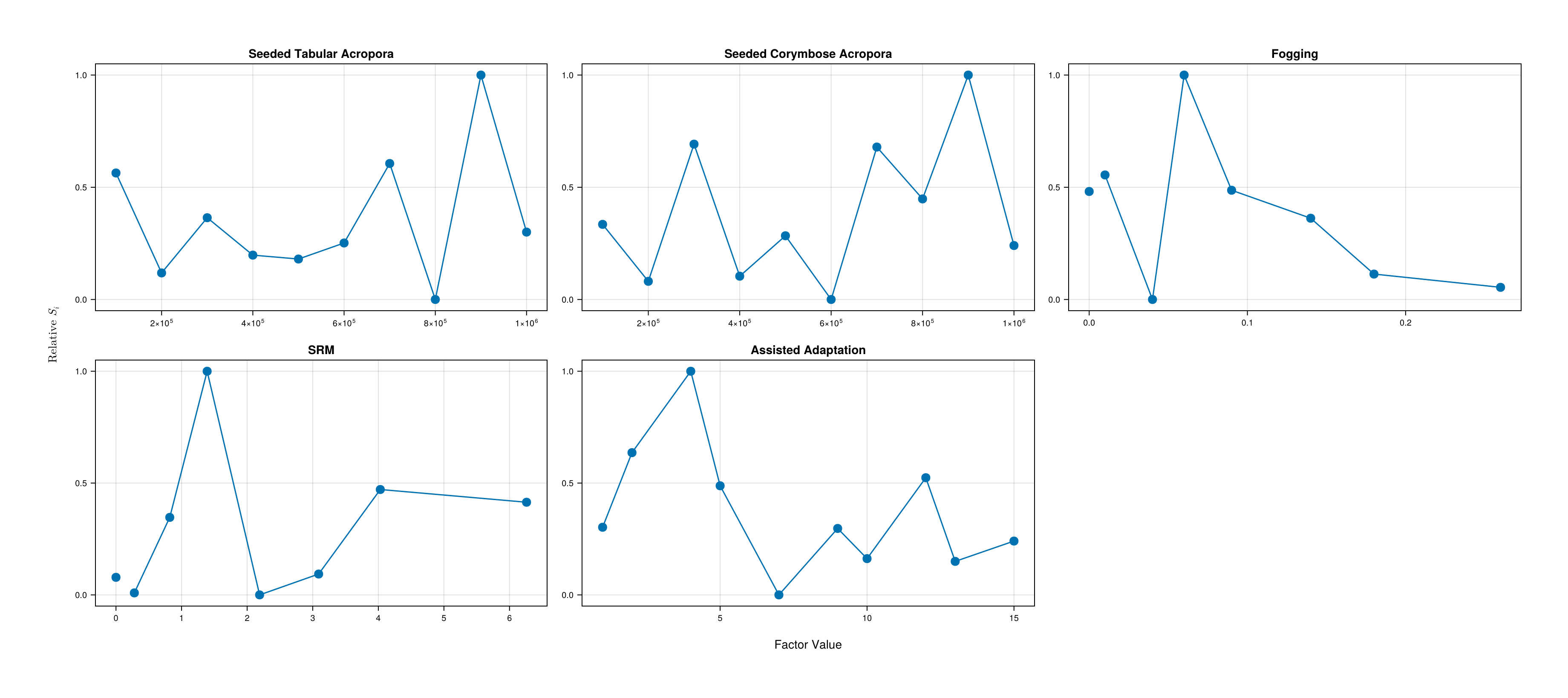

How to read this figure: Each point is one scenario. The x- and y-axes show the sampled values of the two chosen factors; the colour shows the outcome for that scenario (see colorbar). The contour fill interpolates the outcome surface across the factor space, making regional patterns easier to spot.

• Colour gradient along one axis — that factor is the primary driver; the other contributes little on its own.

• Colour gradient diagonal / interaction pattern — both factors jointly influence the outcome; no single factor dominates.

• Uniform colour throughout — neither factor explains much of the outcome variance; look elsewhere in the factor set.

• Sharp colour boundary — a threshold exists: outcomes change abruptly once a factor crosses a particular value.

Outcome mapping

Outcome mapping plots the value of each factor against a scalar outcome, allowing visual identification of which regions of factor space are associated with high or low outcomes. Pass a Vector{Symbol} to plot multiple factors as subplots.

s_tac = ADRIA.metrics.scenario_total_cover(rs)
mean_s_tac = vec(mean(s_tac; dims=1))

X = ADRIA.feature_set(rs)

foi = [:dhw_scenario, :wave_scenario, :N_seed_TA, :N_seed_CA, :fogging, :SRM]

om_fig = ADRIA.viz.outcome_map(X, mean_s_tac, foi)
ADRIA.viz.savefig(om_fig, "outcome_map.html")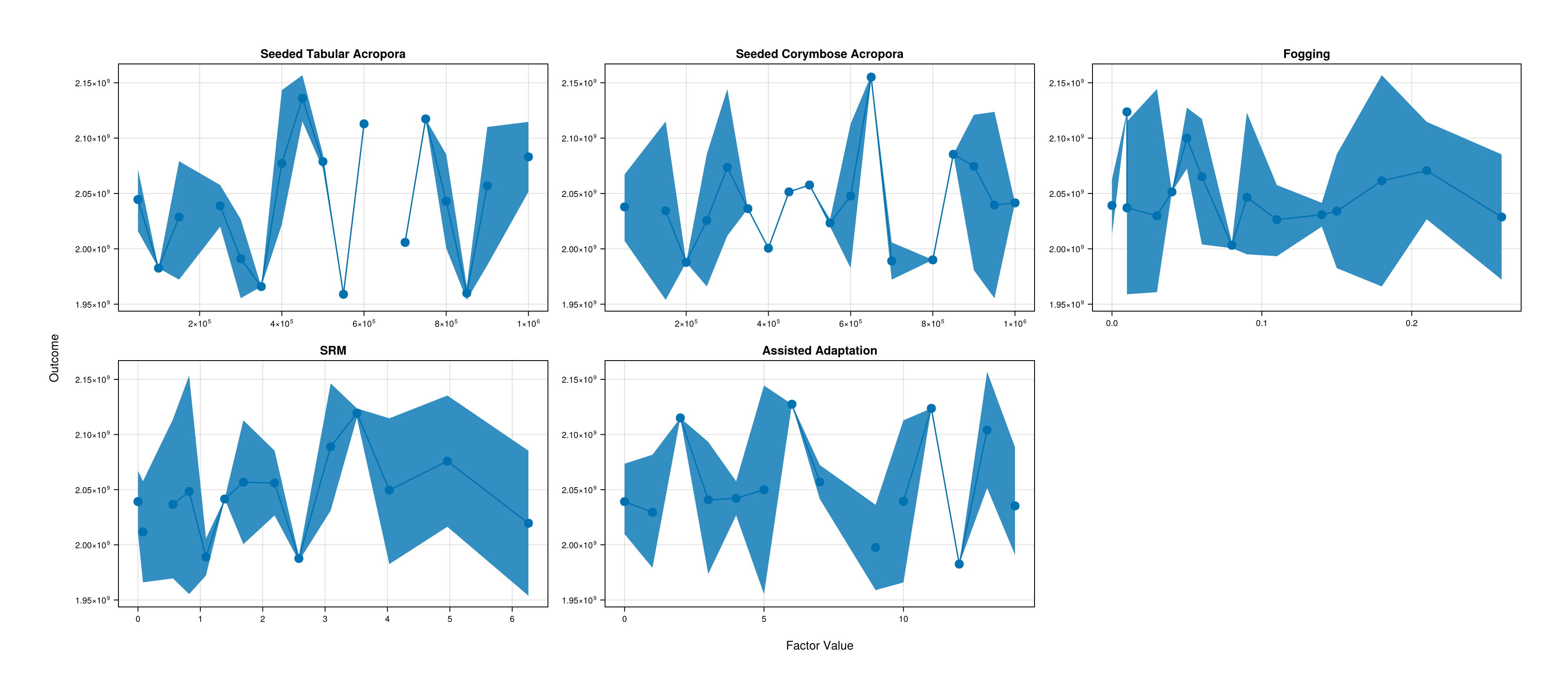

How to read this figure: Each point is one scenario. The x-axis shows the factor value and the y-axis shows the outcome. The density fill (blue shading) shows where scenarios are most concentrated in (factor, outcome) space.

• Density gradient along one axis — the factor positively or negatively influences the outcome; scenarios with higher factor values tend to concentrate at higher or lower outcomes respectively.

• Uniform density across factor values — the factor has little marginal effect on the outcome; other factors are likely more important.

• Wide vertical scatter at any given factor value — high outcome variance that cannot be explained by this factor alone; additional factors must be considered.

• Dense region offset from the bulk — a subset of scenarios cluster away from the main distribution, which may indicate an interaction with another factor.

Feature Ranking

Feature ranking uses the Mann-Whitney U test to score each factor by how well it discriminates between scenarios with high outcomes and all other scenarios. A higher prob_superiority indicates the factor more reliably separates high-outcome scenarios from the rest. effect_size is the rank-biserial correlation.

using ADRIAanalysis

s_tac = ADRIA.metrics.scenario_total_cover(rs)
mean_s_tac = vec(mean(s_tac; dims=1))

X = ADRIA.feature_set(rs)

# Rank-based RSA: score each factor by how well it distinguishes the top 10% of outcomes
ranking = ADRIAanalysis.sensitivity.rsa(X, mean_s_tac)

The returned DataFrame has columns feature, statistic, prob_superiority, and effect_size, sorted descending by prob_superiority.

A selection_mask overload is available for custom outcome filters:

mask = mean_s_tac .>= quantile(mean_s_tac, 0.7)
ranking = ADRIAanalysis.sensitivity.rsa(X, mask)

Data Envelopment Analysis

Performs output-oriented (default, input-oriented can also be applied) Data Envelopment Analysis (DEA) given inputs X and output metrics Y. DEA is used to measure the performance of entities (scenarios), where inputs are converted to outputs via some process. Each scenario's "efficiency score" is calculated relative to an "efficiency frontier", a region representing scenarios for which outputs cannot be further increased by changing inputs (scenario settings).

DEA treats each scenario as a unit that converts inputs into outputs:

• Inputs (X, the "cost") are the resources each scenario consumes and that you want to minimise - for example deployment cost, effort, the number of corals deployed, or the area treated. ADRIA does not prescribe a cost metric: you supply a function (or a precomputed array) that returns one input value per scenario. Pass a Vector{Float64} of length n_scenarios for a single input, or a Matrix{Float64} of size n_scenarios x n_inputs for several. The cost_function in the example below is a placeholder for your own function.

• Outputs (Y) are the benefits each scenario produces and that you want to maximise - metrics such as total coral cover and shelter volume.

The inputs must be row-aligned with the outputs (one row per scenario), strictly positive, and reasonably scaled across scenarios. In particular, avoid inputs that span many orders of magnitude or that approach zero: under the default output orientation a near-zero input against a positive output makes the efficiency frontier unbounded, and the DEA solver will report an infeasible/no-solution status. If "do-nothing" (counterfactual) scenarios are included, give them a meaningful non-zero baseline cost rather than zero.

dom = ADRIA.load_domain("path to domain", "45")

scens = ADRIA.sample(dom, 128)
rs = ADRIA.run_scenarios(dom, scens, "45")

# Compute cost from seeded coral counts; ensure every scenario has a positive baseline
seed_cols = String[c for c in ("N_seed_TA", "N_seed_CA") if c in names(scens)]
cost = if isempty(seed_cols)
    ones(Float64, nrow(scens))
else
    Float64.(vec(sum(Matrix(scens[:, seed_cols]); dims=2))) .+ 1.0
end

# Get mean coral cover and shelter volume for each scenario
s_tac_mean = dropdims(
    mean(ADRIA.metrics.scenario_total_cover(rs); dims=:timesteps); dims=:timesteps
)
asv = ADRIA.metrics.absolute_shelter_volume(rs)
s_sv = dropdims(
    mean(mean(asv; dims=:timesteps); dims=:locations);
    dims=(:timesteps, :locations)
)

# Normalise inputs and outputs to [0, 1] before passing to DEA
function _norm01(v::AbstractVector{Float64})
    lo, hi = extrema(v)
    return hi - lo < eps() ? ones(length(v)) : (v .- lo) ./ (hi - lo)
end

X = _norm01(cost)
Y = hcat(_norm01(Array{Float64}(s_tac_mean)), _norm01(Array{Float64}(s_sv)))

# Output oriented DEA analysis seeking to maximise cover and shelter volume for minimum
# deployment cost
DEA_out = data_envelopment_analysis(X, Y)
dea_fig = ADRIA.viz.data_envelopment_analysis(rs, DEA_out)
ADRIA.viz.savefig(dea_fig, "dea.html")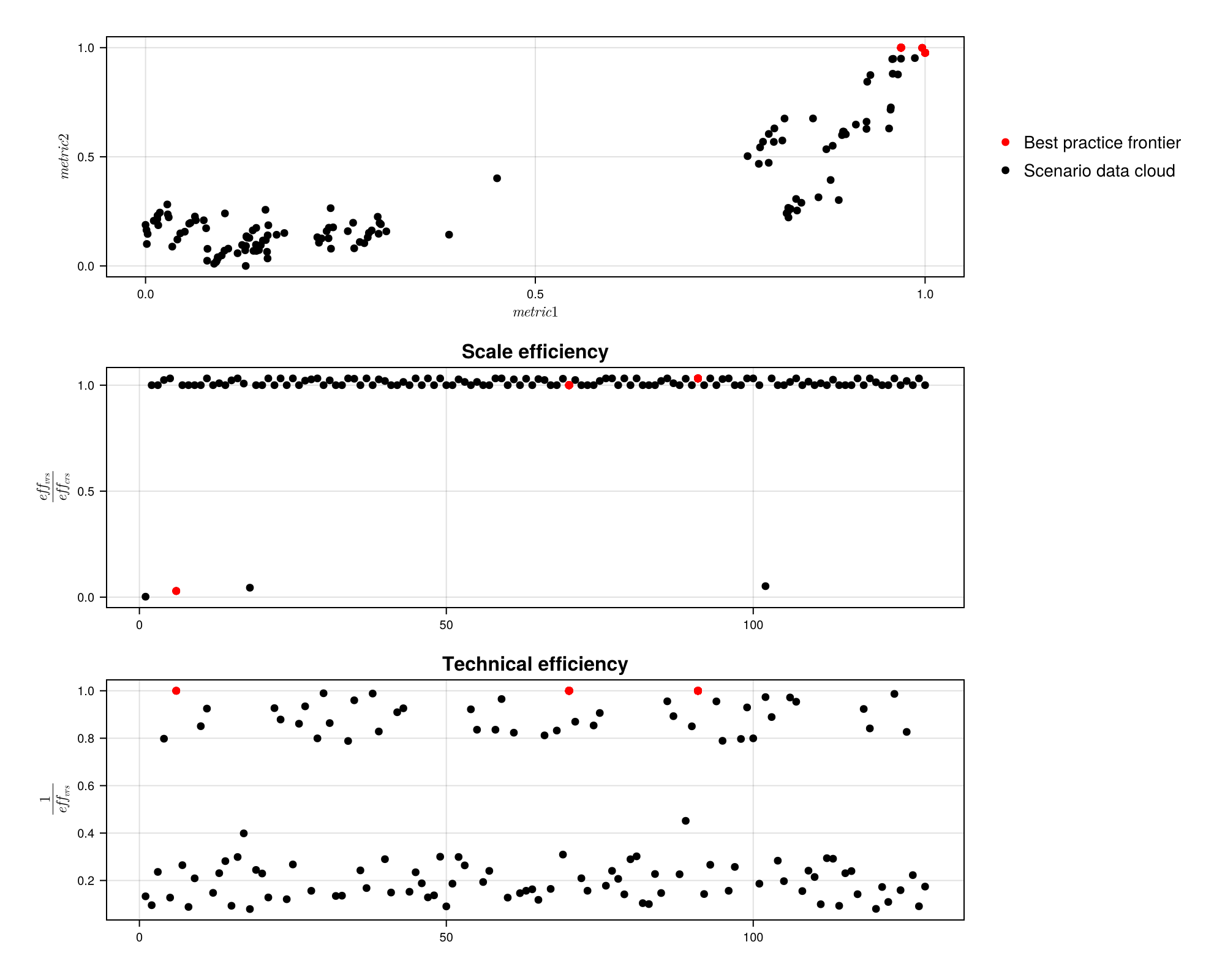

GUI for high-level exploration (prototype only!)

# To explore results interactively
ADRIA.viz.explore("path to Result Set")

# or, if the result set is already loaded:
# ADRIA.viz.explore(rs)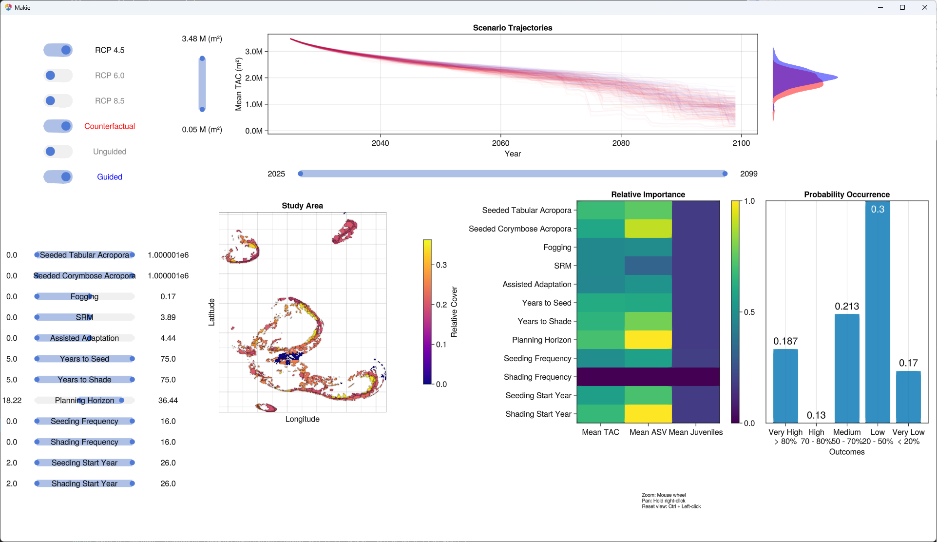

---

This page was generated using Literate.jl.